Large Language Models (LLMs) have taken the world by storm, demonstrating an uncanny ability to understand and generate human language. However, while they excel at grasping general language patterns, achieving specialization in specific domains requires further training. This is where fine-tuning comes in. Fine-tuning LLMs leverages the vast knowledge acquired by LLMs and tailors it towards specialized tasks.
Fine-Tuning LLMs using PEFT
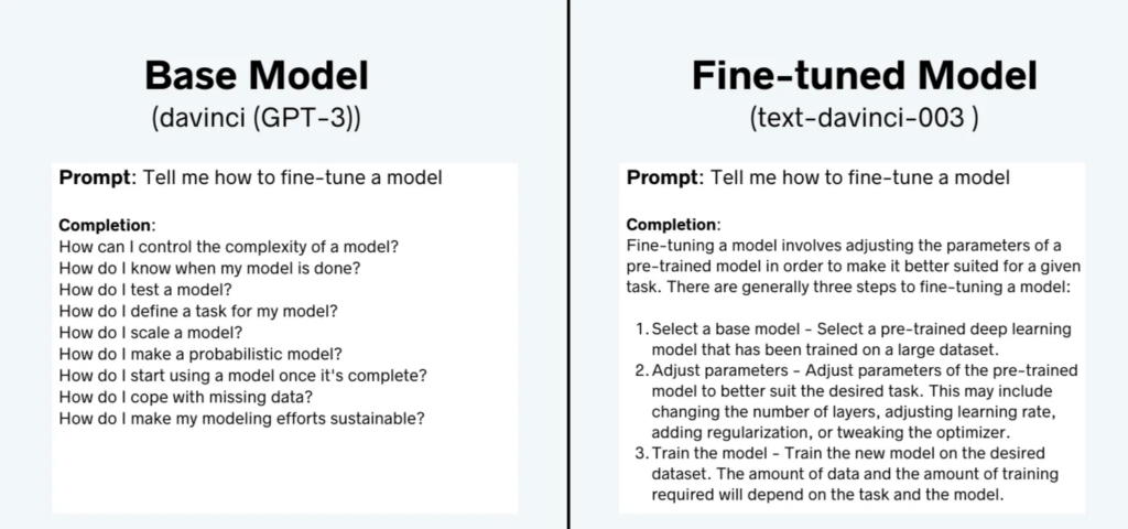
Imagine an LLM pre-trained on a massive corpus of text. It can write different kinds of creative content, translate languages, and answer questions in an informative way. But can it diagnose a disease, write legal contracts, or compose music in a specific style? Not without some focused guidance. Fine-tuning fills this gap, transforming the LLM from a jack-of-all-trades into a domain-specific expert. For example, let’s look at the completions of davinci (GPT-3 base model) and text-davinci-003 (Instruction fine-tuned model).
Figure 1. Completion comparison between a GPT-3 base model and corresponding fine-tuned model.
See the difference? While the base model goes in search mode, the fine-tuned version gives a more helpful and informative response. That’s the power of fine-tuning. By training a model on specific goals and values, we can unlock its true potential. In this article, we will provide a brief overview of popular fine-tuning techniques. Next, we will focus on understanding LoRA (Low-Rank Adaptation) in detail. Subsequently, we will provide a detailed guide, walking through the step-by-step process of fine-tuning a large language model (LLM) for a summarization task utilizing LoRA.
Why Finetune LLMs?
Why bother with fine-tuning when LLMs already seem quite impressive? The answer lies in the power of specialization. Here are some key benefits of fine-tuning LLMs:
- Enhanced Accuracy and Performance: Fine-tuning allows LLMs to delve deeper into the nuances of a specific domain, leading to more accurate and relevant outputs. Imagine a medical LLM trained on medical journals and patient data; its diagnoses could be far more precise than an LLM relying only on general text.
- Reduced Training Time and Resources: Starting with a pre-trained LLM saves a tremendous amount of time and computational resources compared to training from scratch. Think of it as building upon an existing foundation instead of laying a new one.
- Improved Generalizability: While finetuned for a specific task, the LLM retains its ability to adapt and learn within that domain. This enhanced flexibility allows it to handle unseen data and situations more effectively.
- Unlocks LLMs Full Potential: Fine-tuning opens doors to a variety of applications that LLMs are capable of. From personalized education to automated legal research, the possibilities are unlimited.
Fine-tuning not only improves the performance of a base model, but a smaller (finetuned) model can often outperform larger (more expensive) models on the set of tasks on which it was trained. OpenAI demonstrated this with their first generation “InstructGPTˮ models, where the 1.3B parameter InstructGPT model completions were preferred over the 175B parameter GPT-3 base model despite being 100x smaller. This shows the power that fine-tuning offers.
In this article, we will focus on parameter-efficient fine-tuning (PEFT) techniques. To explore full fine-tuning you can check our previous article on Fine Tuning T5.
PEFT Techniques
LLMs can be pretty large, with the largest requiring hundreds of gigabytes of storage. While performing full fine-tuning, the GPU memory requirements are enormous as well. You need to store not only all the model weights but also gradients, optimizer states, forward activations, and temporary states throughout the training process. This can require a substantial amount of computing power, which can be very expensive and impractical to obtain.
In contrast to full fine-tuning, where every model weight is updated during the supervised learning process, parameter-efficient fine-tuning (PEFT) methods only update a small subset of weights. This can be achieved by fine-tuning selected layers or components of the LLM, or by freezing all the LLM weights, adding a small number of new parameters or layers, and updating only the new components. Typically, only 15-20% of the total number of parameters of the LLM are updated, and often, PEFT can be performed using a single GPU.
Since most LLM weights are only slightly modified or left unchanged, the risk of catastrophic forgetting is reduced significantly as well.
The 3 main classes of PEFT methods are as follows:
1. Selective methods: These specialize in fine-tuning just a portion of the initial LLM parameters. You have various options to decide which parameters to modify. You can opt to train specific components of the model, specific layers, or even specific types of parameters.
2. Reparameterization methods: These methods reduce the number of parameters to train by creating new low-rank transformations of the original network weights. One commonly used technique of this type is LoRA, which we will explore in detail in the following sections.
3. Additive methods: These methods perform fine-tuning by keeping the original LLM weights unchanged and incorporating new trainable components. There are two primary approaches in this context. Adapter methods introduce new trainable layers into the model’s architecture, usually within the encoder or decoder components, following the attention or feed-forward layers. Conversely, soft prompt methods maintain the fixed and frozen model architecture while focusing on manipulating the input to enhance performance. This can be achieved by adding trainable parameters to the prompt embeddings or by keeping the input unchanged and retraining the embedding weights.
Adapters
Adapter-based methods add extra trainable parameters after the attention and fully connected layers of a frozen pre-trained model to reduce memory usage and speed up training. The method varies depending on the adapter, it could simply be an extra added layer or it could be expressing the weight updates ∆W as a low-rank decomposition of the weight matrix. Either way, the adapters are typically small but demonstrate comparable performance to a fully finetuned model, enabling training larger models with fewer resources.
There are several ways to express the weight matrix as a low-rank decomposition, but Low-Rank Adaptation (LoRA) is the most common method. There are several other LoRA variants, such as Low-Rank Hadamard Product (LoHa), Low-Rank Kronecker Product (LoKr), and Adaptive Low-Rank Adaptation (AdaLoRA). In this article, we will focus on understanding how LoRA works and how to utilize it to finetune LLMs for your needs.
Soft Prompts
The training of large pre-trained language models (LLMs) presents a significant challenge in terms of both temporal and computational resource investment. As their size continues to grow, researchers are increasingly drawn to more efficient training methods such as prompting. Prompting leverages a pre-trained, frozen model for specific downstream tasks by introducing a textual prompt that either describes the task or offers an illustrative example. This approach eliminates the need to fully train a separate model for each downstream task, allowing for the same frozen pre-trained model to be utilized.
This simplification yields two primary benefits: the model can be readily adapted to handle various tasks, and the training and storage of a smaller set of prompt parameters prove considerably more efficient than training the entirety of the model’s parameters.
Prompting methodologies can be broadly categorized into two distinct groups:
- Hard Prompts: These consist of manually crafted textual prompts composed of discrete input tokens. While this approach offers the advantage of human interpretability, it necessitates significant effort to construct an effective prompt.
- Soft Prompts: These employ learnable tensors concatenated with the input embeddings, permitting optimization based on a specific dataset. The downside is that they aren’t human-readable because you aren’t matching these “virtual tokens” to the embeddings of a real word
A brief overview of the soft prompt methods is given as:
Prompt tuning: It’s like giving your model specific instructions at the start. This means asking it to generate the class label for text classification. The instructions, called prompts, are added to the input as a series of tokens. The key idea behind prompt tuning is that prompt tokens have their parameters that are updated independently. This means you can keep the pre-trained model’s parameters frozen, and only update the gradients of the prompt token embeddings. The results are comparable to the traditional method of training the entire model, and prompt tuning performance scales as model size increases.
Prefix Tuning: It was designed for natural language generation (NLG) tasks on GPT models. It is very similar to prompt tuning; prefix tuning also prepends a sequence of task-specific vectors to the input that can be trained and updated while keeping the rest of the pre-trained model’s parameters frozen.
The main difference is that the prefix parameters are inserted in all of the model layers, whereas prompt tuning only adds the prompt parameters to the model input embeddings. The prefix parameters are also optimized by a separate feed-forward network (FFN) instead of training directly on the soft prompts because it causes instability and degrades performance. The FFN is discarded after updating the soft prompts.
As a result, the authors found that prefix tuning demonstrates comparable performance to fully finetuning a model, despite having 1000x fewer parameters, and it performs even better in low-data settings.
P-tuning: It is designed for natural language understanding (NLU) tasks and all language models. It is another variation of a soft prompt method; P-tuning also adds a trainable embedding tensor that can be optimized to find better prompts, and it uses a prompt encoder (a bidirectional long-short-term memory network or LSTM) to optimize the prompt parameters. Unlike prefix tuning, though:
- The prompt tokens can be inserted anywhere in the input sequence, and it isn’t restricted to only the beginning
- The prompt tokens are only added to the input instead of adding them to every layer of the model
- Introducing anchor tokens can improve performance because they indicate characteristics of a component in the input sequence
The results suggest that P-tuning is more efficient than manually crafting prompts, and it enables GPT-like models to compete with BERT-like models on NLU tasks.
LoRA: An Overview
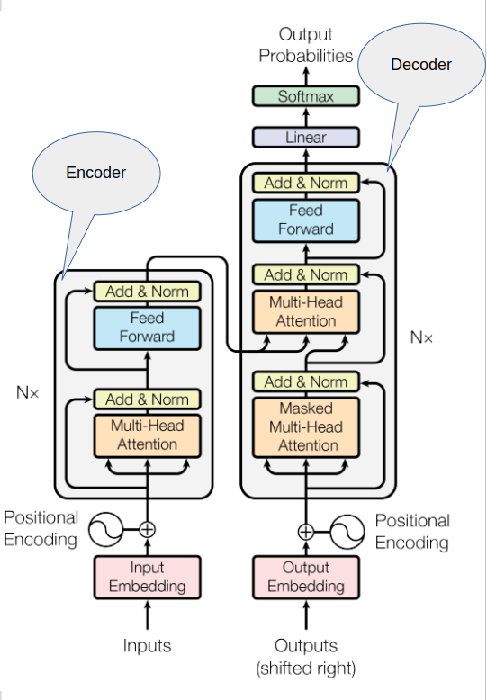
Low-rank Adaptation, or LoRA for short, is a parameter-efficient fine-tuning technique that falls into the re-parameterization category. As a quick reminder, here’s the diagram of the transformer architecture that we saw earlier in Deciphering LLMs: From Transformers to Quantization
Figure 5. Transformer Architecture from this paper.
The input prompt goes through a tokenization process, breaking it into tokens. These tokens are then transformed into embedding vectors, which are subsequently input into the encoder and/or decoder sections of the transformer. Within these components, two types of neural networks operate self-attention and feedforward networks. The weights for these networks are acquired during pre-training.
Once the embedding vectors are generated, they are directed into the self-attention layers. Here, a set of weights is applied to compute attention scores. In the complete fine-tuning process, every parameter in these layers undergoes updates to refine the model
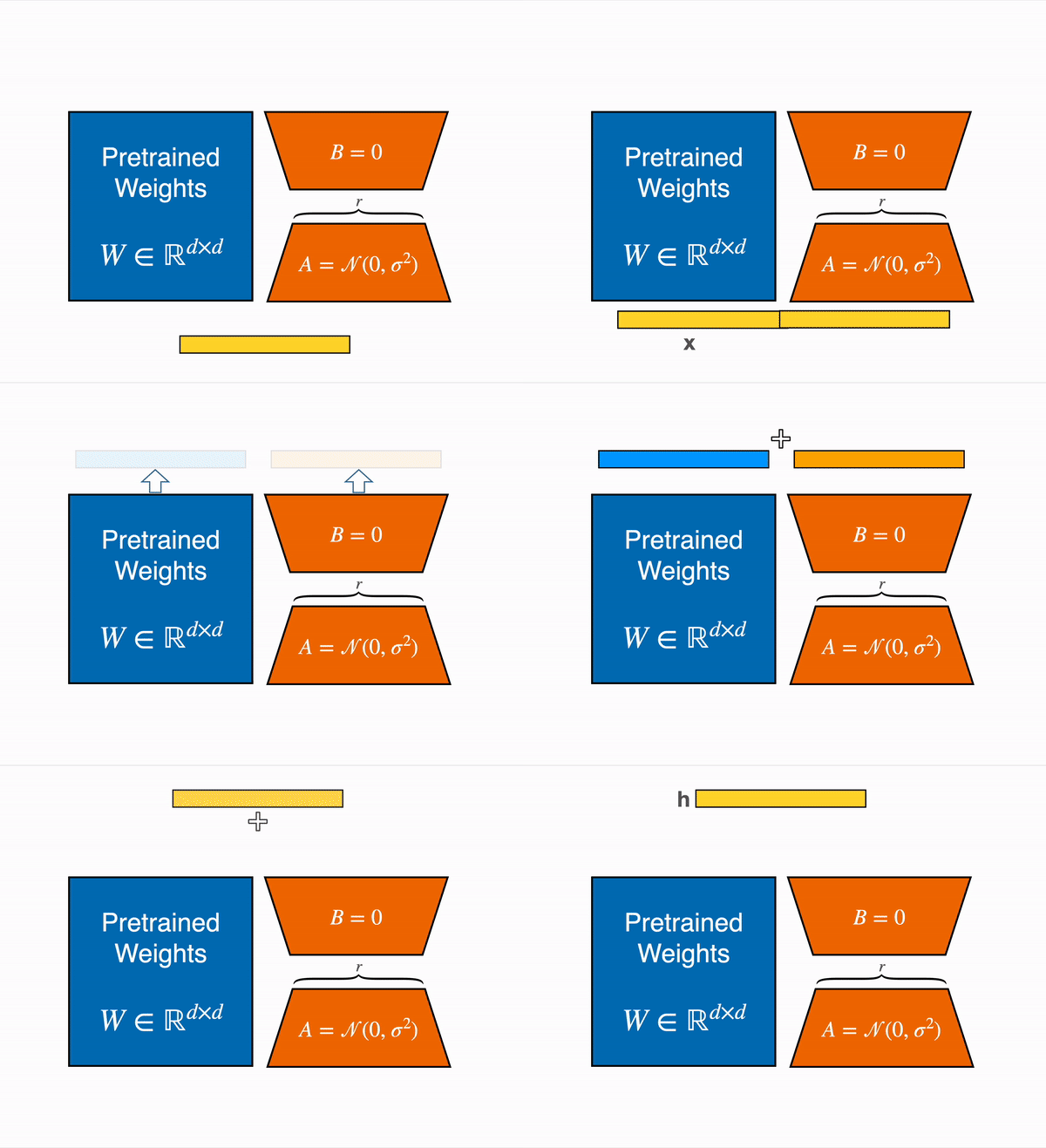
Figure 6. Low-Rank Adapters from this paper.
Figure 7. Low-Rank Matrices.
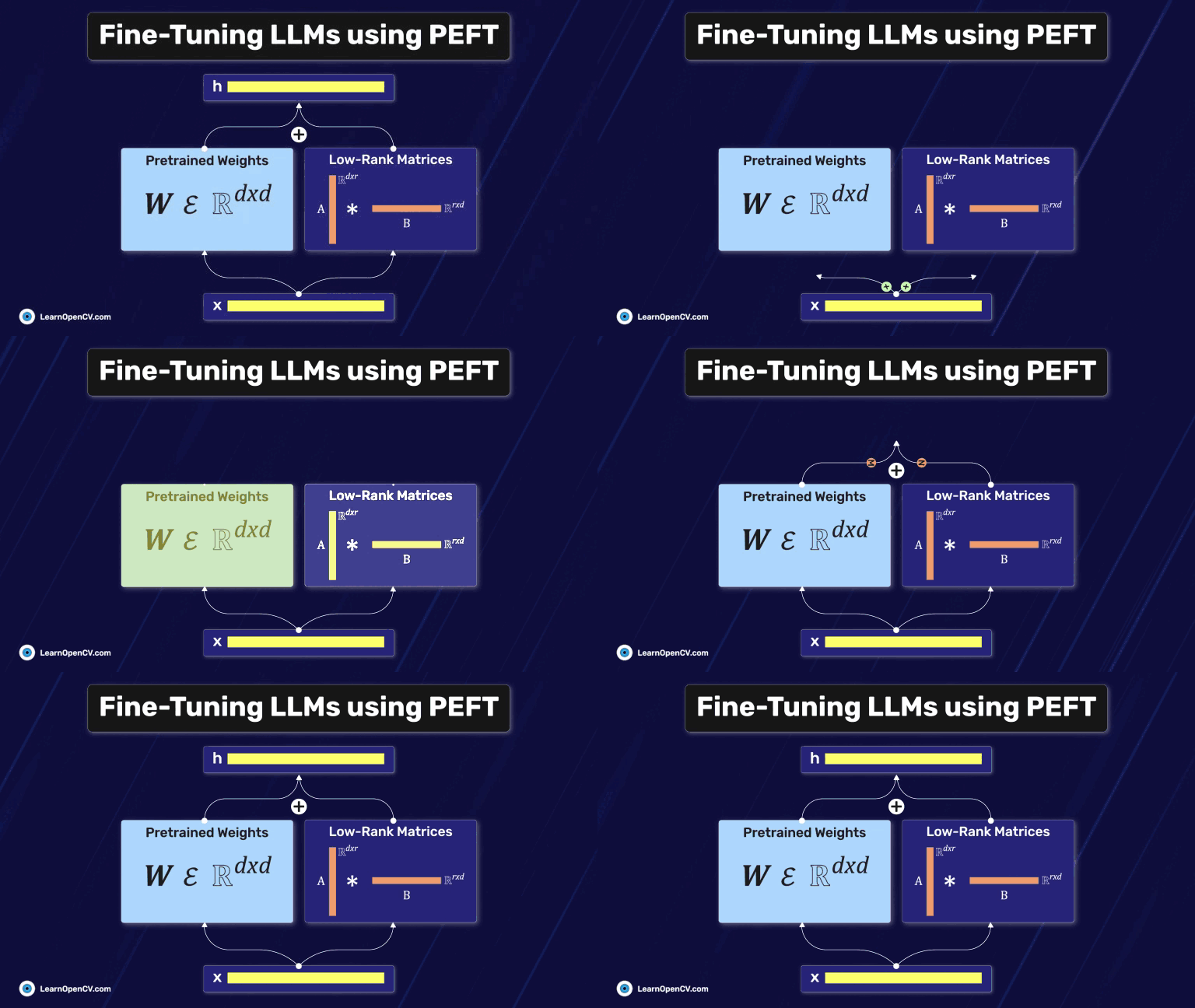
LoRA is a strategy that reduces the number of parameters to be trained during fine-tuning by freezing all of the original model parameters and then injecting a pair of rank decomposition matrices alongside the original weights. The dimensions of the smaller matrices are set so that their product is a matrix with the exact dimensions as the weights they’re modifying. You then keep the original weights of the LLM frozen and train the smaller matrices with supervised learning. For inference, the two low-rank matrices are multiplied to create a matrix with the same dimensions as the frozen weights. You then add this to the original weights and replace them with these updated values in the model.
Researchers have found that applying LoRA to just the self-attention layers of the model is often enough to finetune for a task and achieve performance gains.
Let’s take a practical example using the transformer architecture outlined in the “Attention is All You Need” paper. According to the paper, the transformer weights possess dimensions of 512 by 64, resulting in 32,768 trainable parameters for each weight matrix.
If you employ LoRA as a fine-tuning method with a rank equal to sixteen, you will be training two small rank decomposition matrices with a small dimension of eight. Matrix A will be 64 by 16, summing up to 1024 total parameters. Meanwhile, Matrix B will be 16 by 512, contributing 8,192 trainable parameters. By updating the weights of these new low-rank matrices instead of the original weights, you effectively reduce the training parameters from 32,768 to 9,216 – a substantial 72% reduction.
The beauty of LoRA lies in its ability to significantly diminish the number of trainable parameters. This reduction often allows you to execute parameter-efficient fine-tuning on a single GPU, eliminating the need for a distributed cluster of GPUs. Furthermore, because the rank-decomposition matrices are small, you can finetune a distinct set for each task and switch them out at inference time by updating the weights. This enhances efficiency and provides adaptability for various tasks without compromising performance. But things don’t end just here. We can go a step forward and reduce the memory requirements even further without significantly compromising the performance using QLoRA. Before delving into QLoRA, having a basic understanding of Quantization will be helpful. If you are unfamiliar with it, you can check out the Quantization section in the Deciphering LLMs post.
QLoRA
Building upon the success of LoRA (Low-Rank Adaptation), QLoRA (Quantized Low-Rank Adaptation) introduces two key innovations to further maximize efficiency during fine-tuning of large language models (LLMs):
1. Quantization: While LoRA reduces the number of trainable parameters by representing updates with low-rank matrices, QLoRA adds another layer of optimization. It employs 4-bit NormalFloat (NF4) quantization, an information-theoretically optimal quantization data type for normally distributed data that yields better empirical results than 4-bit Integers and 4-bit Floats. A typical Quantization process consists of converting a data type with more bits to a data type containing fewer bits. To ensure that the entire range of the low-bit data type is used, the input data type is commonly rescaled into the target data type range through normalization by the absolute maximum of the input elements.
For example, quantizing a 32-bit Floating Point (FP32) tensor into an Int8 tensor with range [−127, 127]:
where c is the quantization constant or quantization scale.
The problem with this approach is that if a large magnitude value (i.e., an outlier) occurs in the input tensor, then the quantization bin certain bit combinations are not utilized well with few or no numbers quantized in some bins. To address this issue the NormalFloat (NF) data type builds on Quantile Quantization which is an information-theoretically optimal data type that ensures each quantization bin has an equal number of values assigned from the input tensor. Quantile quantization works by estimating the quantile of the input tensor through the empirical cumulative distribution function. In simple words, the difference between standard and normal float quantization is that the representation here is equally sized rather than equally spaced.
This offers several significant benefits such as significantly reduced (32-bits to 4-bits per parameter) memory requirements, reduced computation, and faster training and inference.
2. Double Quantization: QLoRA takes quantization a step further by employing double quantization. This means not only are the original LLM weights quantized, but also the quantization constants. More specifically, Double Quantization treats quantization constants cFP32 of the first quantization as inputs to a second quantization. This second step yields the quantized quantization constants cFP8. This reduces the memory footprint by 0.373 bits per parameter.
In the author’s own words:
QLoRA, is an efficient finetuning approach that reduces memory usage enough to finetune a 65B parameter model on a single 48GB GPU while preserving full 16-bit finetuning task performance.
This is incredible. To perform full fine-tuning on a 16-bit precision 65B parameter model it would take around 800GB of GPU memory and to get similar performance by using just a single 48GB GPU is just amazing. This shows how powerful QLoRA is.
Fine-tuning LLM using LoRA
In this section, we will finetune a language model on a summarization task and see how it improves the performance of our model. Here, we will finetune google/flan-t5-base model with 248 million parameters using LoRA on samsum dataset. Flan-T5 is an enhanced version of T5 that has been finetuned on multiple tasks, weʼll now use LoRA to finetune this model on summarization tasks further. Finally, we will measure the performance of our finetuned model and the base model using ROUGE metrics.
Download CodeTo easily follow along this tutorial, please download code by clicking on the button below. It's FREE!
Imports
We will start by importing important libraries and modules. Many of the libraries used here are from Hugging Face(HF)
from datasets import load_dataset from transformers import AutoModelForSeq2SeqLM, AutoTokenizer, GenerationConfig, TrainingArguments, Trainer import torch import time import evaluate import pandas as pd import numpy as np
Loading the Base Model
Now we will load our base model. You can load any model of your choice here. You can find the list of models available here. In the second line, we are loading the pre-trained version of google/flan-t5-base model. The torch_dtype parameter specifies the data type you want to load the model weights. The default data type is float32 but we will load the weights using bfloat16 data type, a popular choice for quantization to reduce our computational requirements. Next, we will initialize the tokenizer which was originally used to pre-train the google/flan-t5-base model.
model_name='google/flan-t5-base'
original_model = AutoModelForSeq2SeqLM.from_pretrained(model_name, torch_dtype=torch.bfloat16) tokenizer = AutoTokenizer.from_pretrained(model_name)
Pre-processing the Data
To apply the tokenizer to the dataset, we use the .map() method. This takes in a custom function that specifies how the text should be pre-processed. In this case, that function is called tokenize_function(). We will remove the columns we donʼt need in the next step.
def tokenize_function(example): start_prompt = 'Summarize the following conversation.\n\n' end_prompt = '\n\nSummary: ' prompt = [start_prompt + dialogue + end_prompt for dialogue in example["dialogue"]] example['input_ids'] = tokenizer(prompt, padding="max_length", truncation=True, return_tensors="pt").input_ids example['labels'] = tokenizer(example["summary"], padding="max_length", truncation=True, return_tensors="pt").input_ids
return example
The dataset contains 3 different splits. Tokenize function is handling all of these splits
tokenized_datasets = dataset.map(tokenize_function, batched=True) tokenized_datasets = tokenized_datasets.remove_columns(['id', 'dialogue', 'summary',]) tokenized_datasets = tokenized_datasets.filter(lambda example, index: index % 12 == 0, with_indices=True)
We will use a subset of the original data for fine-tuning.
Fine-tuning with LoRA
First, we will set the configuration parameters for LoRA. More details are provided in the comments. Then, we will initialize the PEFT model using the original model and the LoRA configuration. To get the names of parameters for target_modules you can print the model architecture.
from peft import LoraConfig, get_peft_model, TaskType
Setting up the configuration
lora_config = LoraConfig( r=32, # Rank of the low-rank matrices lora_alpha=32, # Similar to learning rate target_modules=["q", "v"], # Targeting query and key layers lora_dropout=0.05, # Similar to dropout in neural networks bias="none", task_type=TaskType.SEQ_2_SEQ_LM # FLAN-T5 task type )
peft_model = get_peft_model(original_model, lora_config)
Next, we will set the hyper-parameters and other training arguments. Then, we will initialize the trainer instance using our peft_model and training arguments.
output_dir = f'./peft-training-{str(int(time.time()))}'
peft_training_args = TrainingArguments( output_dir=output_dir, auto_find_batch_size=True, # Automatically computes the largest batch size possible learning_rate=1e-3, # Will be higher compared to LR for full finetuning weight_decay=0.01, num_train_epochs=10, logging_steps=50, )
peft_trainer = Trainer( model=peft_model, args=peft_training_args, train_dataset=tokenized_datasets["train"], )
Finally, we will begin the fine-tuning.
time1 = time.time() peft_trainer.train() # Starts the training time2 = time.time()
training_time = time2 - time1
print(f'Time taken to train the model for 10 epochs using LoRA is: {training_time} seconds')
Output:
Time taken to train the model for 10 epochs using LoRA is: 3571.267054080963 seconds
A few outputs are given below:
| Step | Training Loss | | ---- | ------------- | | 1100 | 0.106000 | | 1150 | 0.108600 | | 1200 | 0.106200 | | 1250 | 0.104000 | | 1300 | 0.106500 | | 1350 | 0.107400 | | 1400 | 0.108100 | | 1450 | 0.103000 | | 1500 | 0.106700 |
Evaluation
Next, we will compare the performance of the original model and the finetuned model.
index = 75 dialogue = dataset['test'][index]['dialogue'] baseline_human_summary = dataset['test'][index]['summary']
prompt = f""" Summarize the following conversation.
{dialogue}
Summary: """
input_ids = tokenizer(prompt, return_tensors="pt").input_ids
original_model_outputs = original_model.generate(input_ids=input_ids, generation_config=GenerationConfig(max_new_tokens=200, num_beams=1)) original_model_text_output = tokenizer.decode(original_model_outputs[0], skip_special_tokens=True)
peft_model_outputs = peft_model.generate(input_ids=input_ids, generation_config=GenerationConfig(max_new_tokens=200, num_beams=1)) peft_model_text_output = tokenizer.decode(peft_model_outputs[0], skip_special_tokens=True)
print(f'PROMPT: \n {prompt}') print(dash_line) print(f'BASELINE HUMAN SUMMARY:\n{baseline_human_summary}') print(dash_line) print(f'ORIGINAL MODEL:\n{original_model_text_output}') print(dash_line) print(f'PEFT MODEL:\n {peft_model_text_output}')
'''Output: PROMPT:
Summarize the following conversation.
Steve: BTW, USA won last night! Gulab: I forgot to check! Steve: England playing tomorrow at 2:00! Gulab: That's right, Croatia? Steve: Yep.
Summary:
BASELINE HUMAN SUMMARY: USA won last night. England is playing against Croatia tomorrow at 2.
ORIGINAL MODEL: Steve and Gulab are going to watch England play tomorrow at 2:00.
PEFT MODEL: Steve and Gulab are discussing the USA's win last night. England will play tomorrow at 2:00.'''
You can see that the PEFT model summarized better than the original model. You can play around with different examples and see the results for yourself.
Now, we will use the ROUGE score to compare the performance between the base and fine-tuned models. Here, we are computing the average ROUGE scores over 10 examples. You can vary the number yourself and experiment. To understand more about evaluation metrics you can check out Deciphering LLMs: From Transformers to Quantization
rouge = evaluate.load('rouge')
original_model_results = rouge.compute( predictions=original_model_summaries, # Summaries generated using the base model references=human_baseline_summaries[0:len(original_model_summaries)], # Reference summaries by humans use_aggregator=True, use_stemmer=True, )
peft_model_results = rouge.compute( predictions=peft_model_summaries, # Summaries generated using the fine-tuned model references=human_baseline_summaries[0:len(peft_model_summaries)] # Reference summaries by humans use_aggregator=True, use_stemmer=True, )
print('ORIGINAL MODEL:') print(original_model_results) print('PEFT MODEL:') print(peft_model_results)
''' ORIGINAL MODEL: {'rouge1': 0.42889770784823256, 'rouge2': 0.1705213408281177, 'rougeL': 0.3118532691066424, 'rougeLsum': 0.313564711150918} PEFT MODEL: {'rouge1': 0.468268254301067, 'rouge2': 0.23619570506455861, 'rougeL': 0.39021428273346437, 'rougeLsum': 0.3897312655420616} '''
Notice that the PEFT model results are better than the original model, even after doing full fine-tuning the results would have been more or less the same as the PEFT model results. But performing full fine-tuning would take way more compute resources. If we were to perform full fine-tuning using a single GPU as we did here, it would take us a lot more time to train the model for 10 epochs compared to what it took us here.
Conclusion
In this article we discussed the benefits of fine-tuning pre-trained large language models (LLMs), specifically using LoRA to unlock the true potential of large language models (LLMs). We began by understanding the limitations of general-purpose LLMs and the need for targeted training to specialize in specific domains. This led us to explore the power of fine-tuning, a technique that transforms LLMs into domain experts by focusing on relevant learning.
We delved deeper into Parameter Efficient fine-tuning (PEFT), a game-changer that addresses the resource constraints of traditional fine-tuning by focusing on a smaller subset of parameters. This opens up the opportunity to train LLMs on personal devices or smaller datasets, democratizing access to their capabilities.
Among the various PEFT techniques, we explored LoRA, a powerful method that leverages low-rank adaptations to achieve efficient fine-tuning. We saw how LoRA can be implemented step-by-step on a summarization dataset, demonstrating its ability to significantly improve performance compared to the unadapted LLM. In the next part of the Mastering LLMs series, we will dive into the exciting world of Retrieval-Augmented Generation (RAG) further powering our LLM applications with external knowledge.
Subscribe & Download Code
If you liked this article and would like to download code (C++ and Python) and example images used in this post, please click here. Alternately, sign up to receive a free Computer Vision Resource Guide. In our newsletter, we share OpenCV tutorials and examples written in C++/Python, and Computer Vision and Machine Learning algorithms and news.


