LoRA: Low-Rank Adaptation of Large Language Models

An important paradigm of natural language processing consists of large-scale pre-training on general domain data and adaptation to particular tasks or domains. As we pre-train larger models, full fine-tuning, which retrains all model parameters, becomes less feasible. Using GPT-3 175B as an example – deploying independent instances of fine-tuned models, each with 175B parameters, is prohibitively expensive. We propose Low-Rank Adaptation, or LoRA, which freezes the pre-trained model weights and injects trainable rank decomposition matrices into each layer of the Transformer architecture, greatly reducing the number of trainable parameters for downstream tasks. Compared to GPT-3 175B fine-tuned with Adam, LoRA can reduce the number of trainable parameters by 10,000 times and the GPU memory requirement by 3 times. LoRA performs on-par or better than fine-tuning in model quality on RoBERTa, DeBERTa, GPT-2, and GPT-3, despite having fewer trainable parameters, a higher training throughput, and, unlike adapters, no additional inference latency. We also provide an empirical investigation into rank-deficiency in language model adaptation, which sheds light on the efficacy of LoRA. We release a package that facilitates the integration of LoRA with PyTorch models and provide our implementations and model checkpoints for RoBERTa, DeBERTa, and GPT-2 at https://github.com/microsoft/LoRA.

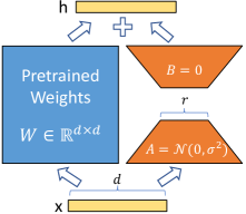
Figure 1: Our reparametrization. We only train A𝐴A and B𝐵B.

Many applications in natural language processing rely on adapting one large-scale, pre-trained language model to multiple downstream applications. Such adaptation is usually done via fine-tuning, which updates all the parameters of the pre-trained model. The major downside of fine-tuning is that the new model contains as many parameters as in the original model. As larger models are trained every few months, this changes from a mere “inconvenience” for GPT-2 (Radford et al., b) or RoBERTa large (Liu et al., 2019) to a critical deployment challenge for GPT-3 (Brown et al., 2020) with 175 billion trainable parameters.

Many sought to mitigate this by adapting only some parameters or learning external modules for new tasks. This way, we only need to store and load a small number of task-specific parameters in addition to the pre-trained model for each task, greatly boosting the operational efficiency when deployed. However, existing techniques often introduce inference latency (Houlsby et al., 2019; Rebuffi et al., 2017) by extending model depth or reduce the model’s usable sequence length (Li & Liang, 2021; Lester et al., 2021; Hambardzumyan et al., 2020; Liu et al., 2021) (Section 3). More importantly, these method often fail to match the fine-tuning baselines, posing a trade-off between efficiency and model quality.

We take inspiration from Li et al. (2018a); Aghajanyan et al. (2020) which show that the learned over-parametrized models in fact reside on a low intrinsic dimension. We hypothesize that the change in weights during model adaptation also has a low “intrinsic rank”, leading to our proposed Low-Rank Adaptation (LoRA) approach. LoRA allows us to train some dense layers in a neural network indirectly by optimizing rank decomposition matrices of the dense layers’ change during adaptation instead, while keeping the pre-trained weights frozen, as shown in Figure 1. Using GPT-3 175B as an example, we show that a very low rank (i.e., r in Figure 1 can be one or two) suffices even when the full rank (i.e., d) is as high as 12,288, making LoRA both storage- and compute-efficient.

LoRA possesses several key advantages.

• •

A pre-trained model can be shared and used to build many small LoRA modules for different tasks. We can freeze the shared model and efficiently switch tasks by replacing the matrices A𝐴A and B𝐵B in [Figure 1](#S1.F1), reducing the storage requirement and task-switching overhead significantly.

• •

LoRA makes training more efficient and lowers the hardware barrier to entry by up to 3 times when using adaptive optimizers since we do not need to calculate the gradients or maintain the optimizer states for most parameters. Instead, we only optimize the injected, much smaller low-rank matrices.

• •

Our simple linear design allows us to merge the trainable matrices with the frozen weights when deployed, introducing no inference latency compared to a fully fine-tuned model, by construction.

• •

LoRA is orthogonal to many prior methods and can be combined with many of them, such as prefix-tuning. We provide an example in [Appendix E](#A5).

We make frequent references to the Transformer architecture and use the conventional terminologies for its dimensions. We call the input and output dimension size of a Transformer layer dm​o​d​e​lsubscript𝑑𝑚𝑜𝑑𝑒𝑙d_{model}. We use Wqsubscript𝑊𝑞W_{q}, Wksubscript𝑊𝑘W_{k}, Wvsubscript𝑊𝑣W_{v}, and Wosubscript𝑊𝑜W_{o} to refer to the query/key/value/output projection matrices in the self-attention module. W𝑊W or W0subscript𝑊0W_{0} refers to a pre-trained weight matrix and Δ​WΔ𝑊\Delta W its accumulated gradient update during adaptation. We use r𝑟r to denote the rank of a LoRA module. We follow the conventions set out by (Vaswani et al., 2017; Brown et al., 2020) and use Adam (Loshchilov & Hutter, 2019; Kingma & Ba, 2017) for model optimization and use a Transformer MLP feedforward dimension df​f​n=4×dm​o​d​e​lsubscript𝑑𝑓𝑓𝑛4subscript𝑑𝑚𝑜𝑑𝑒𝑙d_{ffn}=4\times d_{model}.

While our proposal is agnostic to training objective, we focus on language modeling as our motivating use case. Below is a brief description of the language modeling problem and, in particular, the maximization of conditional probabilities given a task-specific prompt.

Suppose we are given a pre-trained autoregressive language model PΦ​(y|x)subscript𝑃Φconditional𝑦𝑥P_{\Phi}(y|x) parametrized by ΦΦ\Phi. For instance, PΦ​(y|x)subscript𝑃Φconditional𝑦𝑥P_{\Phi}(y|x) can be a generic multi-task learner such as GPT (Radford et al., b; Brown et al., 2020) based on the Transformer architecture (Vaswani et al., 2017). Consider adapting this pre-trained model to downstream conditional text generation tasks, such as summarization, machine reading comprehension (MRC), and natural language to SQL (NL2SQL). Each downstream task is represented by a training dataset of context-target pairs: 𝒵={(xi,yi)}i=1,..,N\mathcal{Z}=\{(x_{i},y_{i})\}_{i=1,..,N}, where both xisubscript𝑥𝑖x_{i} and yisubscript𝑦𝑖y_{i} are sequences of tokens. For example, in NL2SQL, xisubscript𝑥𝑖x_{i} is a natural language query and yisubscript𝑦𝑖y_{i} its corresponding SQL command; for summarization, xisubscript𝑥𝑖x_{i} is the content of an article and yisubscript𝑦𝑖y_{i} its summary.

During full fine-tuning, the model is initialized to pre-trained weights Φ0subscriptΦ0\Phi_{0} and updated to Φ0+Δ​ΦsubscriptΦ0ΔΦ\Phi_{0}+\Delta\Phi by repeatedly following the gradient to maximize the conditional language modeling objective:

maxΦ​∑(x,y)∈𝒵∑t=1|y|log​(PΦ​(yt|x,y<t))subscriptΦsubscript𝑥𝑦𝒵superscriptsubscript𝑡1𝑦logsubscript𝑃Φconditionalsubscript𝑦𝑡𝑥subscript𝑦absent𝑡\displaystyle\max_{\Phi}\sum_{(x,y)\in\mathcal{Z}}\sum_{t=1}^{|y|}\text{log}\left(P_{\Phi}(y_{t}|x,y_{<t})\right)

(1)

One of the main drawbacks for full fine-tuning is that for each downstream task, we learn a different set of parameters Δ​ΦΔΦ\Delta\Phi whose dimension |Δ​Φ|ΔΦ|\Delta\Phi| equals |Φ0|subscriptΦ0|\Phi_{0}|. Thus, if the pre-trained model is large (such as GPT-3 with |Φ0|≈175​ BillionsubscriptΦ0175 Billion|\Phi_{0}|\approx 175\text{~{}Billion}), storing and deploying many independent instances of fine-tuned models can be challenging, if at all feasible.

In this paper, we adopt a more parameter-efficient approach, where the task-specific parameter increment Δ​Φ=Δ​Φ​(Θ)ΔΦΔΦΘ\Delta\Phi=\Delta\Phi(\Theta) is further encoded by a much smaller-sized set of parameters ΘΘ\Theta with |Θ|≪|Φ0|much-less-thanΘsubscriptΦ0|\Theta|\ll|\Phi_{0}|. The task of finding Δ​ΦΔΦ\Delta\Phi thus becomes optimizing over ΘΘ\Theta:

maxΘ​∑(x,y)∈𝒵∑t=1|y|log⁡(pΦ0+Δ​Φ​(Θ)​(yt|x,y<t))subscriptΘsubscript𝑥𝑦𝒵superscriptsubscript𝑡1𝑦subscript𝑝subscriptΦ0ΔΦΘconditionalsubscript𝑦𝑡𝑥subscript𝑦absent𝑡\displaystyle\max_{\Theta}\sum_{(x,y)\in\mathcal{Z}}\sum_{t=1}^{|y|}\log\left({p_{\Phi_{0}+\Delta\Phi(\Theta)}(y_{t}|x,y_{<t}})\right)

(2)

In the subsequent sections, we propose to use a low-rank representation to encode Δ​ΦΔΦ\Delta\Phi that is both compute- and memory-efficient. When the pre-trained model is GPT-3 175B, the number of trainable parameters |Θ|Θ|\Theta| can be as small as 0.01%percent0.010.01\% of |Φ0|subscriptΦ0|\Phi_{0}|.

The problem we set out to tackle is by no means new. Since the inception of transfer learning, dozens of works have sought to make model adaptation more parameter- and compute-efficient. See Section 6 for a survey of some of the well-known works. Using language modeling as an example, there are two prominent strategies when it comes to efficient adaptations: adding adapter layers (Houlsby et al., 2019; Rebuffi et al., 2017; Pfeiffer et al., 2021; Rücklé et al., 2020) or optimizing some forms of the input layer activations (Li & Liang, 2021; Lester et al., 2021; Hambardzumyan et al., 2020; Liu et al., 2021). However, both strategies have their limitations, especially in a large-scale and latency-sensitive production scenario.

There are many variants of adapters. We focus on the original design by Houlsby et al. (2019) which has two adapter layers per Transformer block and a more recent one by  Lin et al. (2020) which has only one per block but with an additional LayerNorm (Ba et al., 2016). While one can reduce the overall latency by pruning layers or exploiting multi-task settings (Rücklé et al., 2020; Pfeiffer et al., 2021), there is no direct ways to bypass the extra compute in adapter layers. This seems like a non-issue since adapter layers are designed to have few parameters (sometimes <<1% of the original model) by having a small bottleneck dimension, which limits the FLOPs they can add. However, large neural networks rely on hardware parallelism to keep the latency low, and adapter layers have to be processed sequentially. This makes a difference in the online inference setting where the batch size is typically as small as one. In a generic scenario without model parallelism, such as running inference on GPT-2 (Radford et al., b) medium on a single GPU, we see a noticeable increase in latency when using adapters, even with a very small bottleneck dimension (Table 1).

Batch Size

32

16

1

Sequence Length

512

256

128

|Θ|Θ|\Theta|

0.5M

11M

11M

Fine-Tune/LoRA

1449.4±plus-or-minus\pm0.8

338.0±plus-or-minus\pm0.6

19.8±plus-or-minus\pm2.7

AdapterLsuperscriptAdapterL\text{Adapter}^{\text{L}}

1482.0±plus-or-minus\pm1.0 (+2.2%)

354.8±plus-or-minus\pm0.5 (+5.0%)

23.9±plus-or-minus\pm2.1 (+20.7%)

AdapterHsuperscriptAdapterH\text{Adapter}^{\text{H}}

1492.2±plus-or-minus\pm1.0 (+3.0%)

366.3±plus-or-minus\pm0.5 (+8.4%)

25.8±plus-or-minus\pm2.2 (+30.3%)

Table 1: Infernece latency of a single forward pass in GPT-2 medium measured in milliseconds, averaged over 100 trials. We use an NVIDIA Quadro RTX8000. “|Θ|Θ|\Theta|” denotes the number of trainable parameters in adapter layers. AdapterLsuperscriptAdapterL\text{Adapter}^{\text{L}} and AdapterHsuperscriptAdapterH\text{Adapter}^{\text{H}} are two variants of adapter tuning, which we describe in Section 5.1. The inference latency introduced by adapter layers can be significant in an online, short-sequence-length scenario. See the full study in Appendix B.

This problem gets worse when we need to shard the model as done in Shoeybi et al. (2020); Lepikhin et al. (2020), because the additional depth requires more synchronous GPU operations such as AllReduce and Broadcast, unless we store the adapter parameters redundantly many times.

The other direction, as exemplified by prefix tuning (Li & Liang, 2021), faces a different challenge. We observe that prefix tuning is difficult to optimize and that its performance changes non-monotonically in trainable parameters, confirming similar observations in the original paper. More fundamentally, reserving a part of the sequence length for adaptation necessarily reduces the sequence length available to process a downstream task, which we suspect makes tuning the prompt less performant compared to other methods. We defer the study on task performance to Section 5.

We describe the simple design of LoRA and its practical benefits. The principles outlined here apply to any dense layers in deep learning models, though we only focus on certain weights in Transformer language models in our experiments as the motivating use case.

A neural network contains many dense layers which perform matrix multiplication. The weight matrices in these layers typically have full-rank. When adapting to a specific task, Aghajanyan et al. (2020) shows that the pre-trained language models have a low “instrisic dimension” and can still learn efficiently despite a random projection to a smaller subspace. Inspired by this, we hypothesize the updates to the weights also have a low “intrinsic rank” during adaptation. For a pre-trained weight matrix W0∈ℝd×ksubscript𝑊0superscriptℝ𝑑𝑘W_{0}\in\mathbb{R}^{d\times k}, we constrain its update by representing the latter with a low-rank decomposition W0+Δ​W=W0+B​Asubscript𝑊0Δ𝑊subscript𝑊0𝐵𝐴W_{0}+\Delta W=W_{0}+BA, where B∈ℝd×r,A∈ℝr×kformulae-sequence𝐵superscriptℝ𝑑𝑟𝐴superscriptℝ𝑟𝑘B\in\mathbb{R}^{d\times r},A\in\mathbb{R}^{r\times k}, and the rank r≪min⁡(d,k)much-less-than𝑟𝑑𝑘r\ll\min(d,k). During training, W0subscript𝑊0W_{0} is frozen and does not receive gradient updates, while A𝐴A and B𝐵B contain trainable parameters. Note both W0subscript𝑊0W_{0} and Δ​W=B​AΔ𝑊𝐵𝐴\Delta W=BA are multiplied with the same input, and their respective output vectors are summed coordinate-wise. For h=W0​xℎsubscript𝑊0𝑥h=W_{0}x, our modified forward pass yields:

h=W0​x+Δ​W​x=W0​x+B​A​xℎsubscript𝑊0𝑥Δ𝑊𝑥subscript𝑊0𝑥𝐵𝐴𝑥h=W_{0}x+\Delta Wx=W_{0}x+BAx

(3)

We illustrate our reparametrization in Figure 1. We use a random Gaussian initialization for A𝐴A and zero for B𝐵B, so Δ​W=B​AΔ𝑊𝐵𝐴\Delta W=BA is zero at the beginning of training. We then scale Δ​W​xΔ𝑊𝑥\Delta Wx by αr𝛼𝑟\frac{\alpha}{r}, where α𝛼\alpha is a constant in r𝑟r. When optimizing with Adam, tuning α𝛼\alpha is roughly the same as tuning the learning rate if we scale the initialization appropriately. As a result, we simply set α𝛼\alpha to the first r𝑟r we try and do not tune it. This scaling helps to reduce the need to retune hyperparameters when we vary r𝑟r (Yang & Hu, 2021).

A Generalization of Full Fine-tuning.   A more general form of fine-tuning allows the training of a subset of the pre-trained parameters. LoRA takes a step further and does not require the accumulated gradient update to weight matrices to have full-rank during adaptation. This means that when applying LoRA to all weight matrices and training all biases, we roughly recover the expressiveness of full fine-tuning by setting the LoRA rank r𝑟r to the rank of the pre-trained weight matrices. In other words, as we increase the number of trainable parameters , training LoRA roughly converges to training the original model, while adapter-based methods converges to an MLP and prefix-based methods to a model that cannot take long input sequences.

No Additional Inference Latency.   When deployed in production, we can explicitly compute and store W=W0+B​A𝑊subscript𝑊0𝐵𝐴W=W_{0}+BA and perform inference as usual. Note that both W0subscript𝑊0W_{0} and B​A𝐵𝐴BA are in ℝd×ksuperscriptℝ𝑑𝑘\mathbb{R}^{d\times k}. When we need to switch to another downstream task, we can recover W0subscript𝑊0W_{0} by subtracting B​A𝐵𝐴BA and then adding a different B′​A′superscript𝐵′superscript𝐴′B^{\prime}A^{\prime}, a quick operation with very little memory overhead. Critically, this guarantees that we do not introduce any additional latency during inference compared to a fine-tuned model by construction.

In principle, we can apply LoRA to any subset of weight matrices in a neural network to reduce the number of trainable parameters. In the Transformer architecture, there are four weight matrices in the self-attention module (Wq,Wk,Wv,Wosubscript𝑊𝑞subscript𝑊𝑘subscript𝑊𝑣subscript𝑊𝑜W_{q},W_{k},W_{v},W_{o}) and two in the MLP module. We treat Wqsubscript𝑊𝑞W_{q} (or Wksubscript𝑊𝑘W_{k}, Wvsubscript𝑊𝑣W_{v}) as a single matrix of dimension dm​o​d​e​l×dm​o​d​e​lsubscript𝑑𝑚𝑜𝑑𝑒𝑙subscript𝑑𝑚𝑜𝑑𝑒𝑙d_{model}\times d_{model}, even though the output dimension is usually sliced into attention heads. We limit our study to only adapting the attention weights for downstream tasks and freeze the MLP modules (so they are not trained in downstream tasks) both for simplicity and parameter-efficiency.We further study the effect on adapting different types of attention weight matrices in a Transformer in Section 7.1. We leave the empirical investigation of adapting the MLP layers, LayerNorm layers, and biases to a future work.

Practical Benefits and Limitations.   The most significant benefit comes from the reduction in memory and storage usage. For a large Transformer trained with Adam, we reduce that VRAM usage by up to 2/3232/3 if r≪dm​o​d​e​lmuch-less-than𝑟subscript𝑑𝑚𝑜𝑑𝑒𝑙r\ll d_{model} as we do not need to store the optimizer states for the frozen parameters. On GPT-3 175B, we reduce the VRAM consumption during training from 1.2TB to 350GB. With r=4𝑟4r=4 and only the query and value projection matrices being adapted, the checkpoint size is reduced by roughly 10,000×\times (from 350GB to 35MB). This allows us to train with significantly fewer GPUs and avoid I/O bottlenecks. Another benefit is that we can switch between tasks while deployed at a much lower cost by only swapping the LoRA weights as opposed to all the parameters. This allows for the creation of many customized models that can be swapped in and out on the fly on machines that store the pre-trained weights in VRAM. We also observe a 25% speedup during training on GPT-3 175B compared to full fine-tuning as we do not need to calculate the gradient for the vast majority of the parameters.

LoRA also has its limitations. For example, it is not straightforward to batch inputs to different tasks with different A𝐴A and B𝐵B in a single forward pass, if one chooses to absorb A𝐴A and B𝐵B into W𝑊W to eliminate additional inference latency. Though it is possible to not merge the weights and dynamically choose the LoRA modules to use for samples in a batch for scenarios where latency is not critical.

We evaluate the downstream task performance of LoRA on RoBERTa (Liu et al., 2019), DeBERTa (He et al., 2021), and GPT-2 (Radford et al., b), before scaling up to GPT-3 175B (Brown et al., 2020). Our experiments cover a wide range of tasks, from natural language understanding (NLU) to generation (NLG). Specifically, we evaluate on the GLUE (Wang et al., 2019) benchmark for RoBERTa and DeBERTa. We follow the setup of Li & Liang (2021) on GPT-2 for a direct comparison and add WikiSQL (Zhong et al., 2017) (NL to SQL queries) and SAMSum (Gliwa et al., 2019) (conversation summarization) for large-scale experiments on GPT-3. See Appendix C for more details on the datasets we use. We use NVIDIA Tesla V100 for all experiments.

To compare with other baselines broadly, we replicate the setups used by prior work and reuse their reported numbers whenever possible. This, however, means that some baselines might only appear in certain experiments.

Fine-Tuning (FT) is a common approach for adaptation. During fine-tuning, the model is initialized to the pre-trained weights and biases, and all model parameters undergo gradient updates.A simple variant is to update only some layers while freezing others. We include one such baseline reported in prior work (Li & Liang, 2021) on GPT-2, which adapts just the last two layers (FTTop2superscriptFTTop2\textbf{FT}^{\textbf{Top2}}).

Bias-only or BitFit is a baseline where we only train the bias vectors while freezing everything else. Contemporarily, this baseline has also been studied by BitFit (Zaken et al., 2021).

Prefix-embedding tuning (PreEmbed) inserts special tokens among the input tokens. These special tokens have trainable word embeddings and are generally not in the model’s vocabulary. Where to place such tokens can have an impact on performance. We focus on “prefixing”, which prepends such tokens to the prompt, and “infixing”, which appends to the prompt; both are discussed in Li & Liang (2021). We use lpsubscript𝑙𝑝l_{p} (resp. lisubscript𝑙𝑖l_{i}) denote the number of prefix (resp. infix) tokens. The number of trainable parameters is |Θ|=dm​o​d​e​l×(lp+li)Θsubscript𝑑𝑚𝑜𝑑𝑒𝑙subscript𝑙𝑝subscript𝑙𝑖|\Theta|=d_{model}\times(l_{p}+l_{i}).

Prefix-layer tuning (PreLayer) is an extension to prefix-embedding tuning. Instead of just learning the word embeddings (or equivalently, the activations after the embedding layer) for some special tokens, we learn the activations after every Transformer layer. The activations computed from previous layers are simply replaced by trainable ones. The resulting number of trainable parameters is |Θ|=L×dm​o​d​e​l×(lp+li)Θ𝐿subscript𝑑𝑚𝑜𝑑𝑒𝑙subscript𝑙𝑝subscript𝑙𝑖|\Theta|=L\times d_{model}\times(l_{p}+l_{i}), where L𝐿L is the number of Transformer layers.

Adapter tuning as proposed in Houlsby et al. (2019) inserts adapter layers between the self-attention module (and the MLP module) and the subsequent residual connection. There are two fully connected layers with biases in an adapter layer with a nonlinearity in between. We call this original design AdapterHsuperscriptAdapterH\textbf{Adapter}^{\textbf{H}}. Recently, Lin et al. (2020) proposed a more efficient design with the adapter layer applied only after the MLP module and after a LayerNorm. We call it AdapterLsuperscriptAdapterL\textbf{Adapter}^{\textbf{L}}. This is very similar to another deign proposed in Pfeiffer et al. (2021), which we call AdapterPsuperscriptAdapterP\textbf{Adapter}^{\textbf{P}}. We also include another baseline call AdapterDrop (Rücklé et al., 2020) which drops some adapter layers for greater efficiency (AdapterDsuperscriptAdapterD\textbf{Adapter}^{\textbf{D}}). We cite numbers from prior works whenever possible to maximize the number of baselines we compare with; they are in rows with an asterisk (*) in the first column. In all cases, we have |Θ|=L^A​d​p​t×(2×dm​o​d​e​l×r+r+dm​o​d​e​l)+2×L^L​N×dm​o​d​e​lΘsubscript^𝐿𝐴𝑑𝑝𝑡2subscript𝑑𝑚𝑜𝑑𝑒𝑙𝑟𝑟subscript𝑑𝑚𝑜𝑑𝑒𝑙2subscript^𝐿𝐿𝑁subscript𝑑𝑚𝑜𝑑𝑒𝑙|\Theta|=\hat{L}_{Adpt}\times(2\times d_{model}\times r+r+d_{model})+2\times\hat{L}_{LN}\times d_{model} where L^A​d​p​tsubscript^𝐿𝐴𝑑𝑝𝑡\hat{L}_{Adpt} is the number of adapter layers and L^L​Nsubscript^𝐿𝐿𝑁\hat{L}_{LN} the number of trainable LayerNorms (e.g., in AdapterLsuperscriptAdapterL\text{Adapter}^{\text{L}}).

LoRA adds trainable pairs of rank decomposition matrices in parallel to existing weight matrices. As mentioned in Section 4.2, we only apply LoRA to Wqsubscript𝑊𝑞W_{q} and Wvsubscript𝑊𝑣W_{v} in most experiments for simplicity. The number of trainable parameters is determined by the rank r𝑟r and the shape of the original weights: |Θ|=2×L^L​o​R​A×dm​o​d​e​l×rΘ2subscript^𝐿𝐿𝑜𝑅𝐴subscript𝑑𝑚𝑜𝑑𝑒𝑙𝑟|\Theta|=2\times\hat{L}_{LoRA}\times d_{model}\times r, where L^L​o​R​Asubscript^𝐿𝐿𝑜𝑅𝐴\hat{L}_{LoRA} is the number of weight matrices we apply LoRA to.

Model & Method

# Trainable

Parameters

MNLI

SST-2

MRPC

CoLA

QNLI

QQP

RTE

STS-B

Avg.

RoBbasesubscriptRoBbase\text{RoB}_{\text{base}} (FT)*

125.0M

87.6

94.8

90.2

63.6

92.8

91.9

78.7

91.2

86.4

RoBbasesubscriptRoBbase\text{RoB}_{\text{base}} (BitFit)*

0.1M

84.7

93.7

92.7

62.0

91.8

84.0

81.5

90.8

85.2

RoBbasesubscriptRoBbase\text{RoB}_{\text{base}} (AdptDsuperscriptAdptD\text{Adpt}^{\text{D}})*

0.3M

87.1±plus-or-minus\pm.0

94.2±plus-or-minus\pm.1

88.5±plus-or-minus\pm1.1

60.8±plus-or-minus\pm.4

93.1±plus-or-minus\pm.1

90.2±plus-or-minus\pm.0

71.5±plus-or-minus\pm2.7

89.7±plus-or-minus\pm.3

84.4

RoBbasesubscriptRoBbase\text{RoB}_{\text{base}} (AdptDsuperscriptAdptD\text{Adpt}^{\text{D}})*

0.9M

87.3±plus-or-minus\pm.1

94.7±plus-or-minus\pm.3

88.4±plus-or-minus\pm.1

62.6±plus-or-minus\pm.9

93.0±plus-or-minus\pm.2

90.6±plus-or-minus\pm.0

75.9±plus-or-minus\pm2.2

90.3±plus-or-minus\pm.1

85.4

RoBbasesubscriptRoBbase\text{RoB}_{\text{base}} (LoRA)

0.3M

87.5±plus-or-minus\pm.3

95.1±plus-or-minus\pm.2

89.7±plus-or-minus\pm.7

63.4±plus-or-minus\pm1.2

93.3±plus-or-minus\pm.3

90.8±plus-or-minus\pm.1

86.6±plus-or-minus\pm.7

91.5±plus-or-minus\pm.2

87.2

RoBlargesubscriptRoBlarge\text{RoB}_{\text{large}} (FT)*

355.0M

90.2

96.4

90.9

68.0

94.7

92.2

86.6

92.4

88.9

RoBlargesubscriptRoBlarge\text{RoB}_{\text{large}} (LoRA)

0.8M

90.6±plus-or-minus\pm.2

96.2±plus-or-minus\pm.5

90.9±plus-or-minus\pm1.2

68.2±plus-or-minus\pm1.9

94.9±plus-or-minus\pm.3

91.6±plus-or-minus\pm.1

87.4±plus-or-minus\pm2.5

92.6±plus-or-minus\pm.2

89.0

RoBlargesubscriptRoBlarge\text{RoB}_{\text{large}} (AdptPsuperscriptAdptP\text{Adpt}^{\text{P}})††\dagger

3.0M

90.2±plus-or-minus\pm.3

96.1±plus-or-minus\pm.3

90.2±plus-or-minus\pm.7

68.3±plus-or-minus\pm1.0

94.8±plus-or-minus\pm.2

91.9±plus-or-minus\pm.1

83.8±plus-or-minus\pm2.9

92.1±plus-or-minus\pm.7

88.4

RoBlargesubscriptRoBlarge\text{RoB}_{\text{large}} (AdptPsuperscriptAdptP\text{Adpt}^{\text{P}})††\dagger

0.8M

90.5±plus-or-minus\pm.3

96.6±plus-or-minus\pm.2

89.7±plus-or-minus\pm1.2

67.8±plus-or-minus\pm2.5

94.8±plus-or-minus\pm.3

91.7±plus-or-minus\pm.2

80.1±plus-or-minus\pm2.9

91.9±plus-or-minus\pm.4

87.9

RoBlargesubscriptRoBlarge\text{RoB}_{\text{large}} (AdptHsuperscriptAdptH\text{Adpt}^{\text{H}})††\dagger

6.0M

89.9±plus-or-minus\pm.5

96.2±plus-or-minus\pm.3

88.7±plus-or-minus\pm2.9

66.5±plus-or-minus\pm4.4

94.7±plus-or-minus\pm.2

92.1±plus-or-minus\pm.1

83.4±plus-or-minus\pm1.1

91.0±plus-or-minus\pm1.7

87.8

RoBlargesubscriptRoBlarge\text{RoB}_{\text{large}} (AdptHsuperscriptAdptH\text{Adpt}^{\text{H}})††\dagger

0.8M

90.3±plus-or-minus\pm.3

96.3±plus-or-minus\pm.5

87.7±plus-or-minus\pm1.7

66.3±plus-or-minus\pm2.0

94.7±plus-or-minus\pm.2

91.5±plus-or-minus\pm.1

72.9±plus-or-minus\pm2.9

91.5±plus-or-minus\pm.5

86.4

RoBlargesubscriptRoBlarge\text{RoB}_{\text{large}} (LoRA)††\dagger

0.8M

90.6±plus-or-minus\pm.2

96.2±plus-or-minus\pm.5

90.2±plus-or-minus\pm1.0

68.2±plus-or-minus\pm1.9

94.8±plus-or-minus\pm.3

91.6±plus-or-minus\pm.2

85.2±plus-or-minus\pm1.1

92.3±plus-or-minus\pm.5

88.6

DeBXXLsubscriptDeBXXL\text{DeB}_{\text{XXL}} (FT)*

1500.0M

91.8

97.2

92.0

72.0

96.0

92.7

93.9

92.9

91.1

DeBXXLsubscriptDeBXXL\text{DeB}_{\text{XXL}} (LoRA)

4.7M

91.9±plus-or-minus\pm.2

96.9±plus-or-minus\pm.2

92.6±plus-or-minus\pm.6

72.4±plus-or-minus\pm1.1

96.0±plus-or-minus\pm.1

92.9±plus-or-minus\pm.1

94.9±plus-or-minus\pm.4

93.0±plus-or-minus\pm.2

91.3

Table 2: RoBERTabasesubscriptRoBERTabase\text{RoBERTa}_{\text{base}}, RoBERTalargesubscriptRoBERTalarge\text{RoBERTa}_{\text{large}}, and DeBERTaXXLsubscriptDeBERTaXXL\text{DeBERTa}_{\text{XXL}} with different adaptation methods on the GLUE benchmark. We report the overall (matched and mismatched) accuracy for MNLI, Matthew’s correlation for CoLA, Pearson correlation for STS-B, and accuracy for other tasks. Higher is better for all metrics. * indicates numbers published in prior works. ††\dagger indicates runs configured in a setup similar to Houlsby et al. (2019) for a fair comparison.

RoBERTa (Liu et al., 2019) optimized the pre-training recipe originally proposed in BERT (Devlin et al., 2019a) and boosted the latter’s task performance without introducing many more trainable parameters. While RoBERTa has been overtaken by much larger models on NLP leaderboards such as the GLUE benchmark (Wang et al., 2019) in recent years, it remains a competitive and popular pre-trained model for its size among practitioners. We take the pre-trained RoBERTa base (125M) and RoBERTa large (355M) from the HuggingFace Transformers library (Wolf et al., 2020) and evaluate the performance of different efficient adaptation approaches on tasks from the GLUE benchmark. We also replicate Houlsby et al. (2019) and Pfeiffer et al. (2021) according to their setup. To ensure a fair comparison, we make two crucial changes to how we evaluate LoRA when comparing with adapters. First, we use the same batch size for all tasks and use a sequence length of 128 to match the adapter baselines. Second, we initialize the model to the pre-trained model for MRPC, RTE, and STS-B, not a model already adapted to MNLI like the fine-tuning baseline. Runs following this more restricted setup from Houlsby et al. (2019) are labeled with ††\dagger. The result is presented in Table 2 (Top Three Sections). See Section D.1 for details on the hyperparameters used.

DeBERTa (He et al., 2021) is a more recent variant of BERT that is trained on a much larger scale and performs very competitively on benchmarks such as GLUE (Wang et al., 2019) and SuperGLUE (Wang et al., 2020). We evaluate if LoRA can still match the performance of a fully fine-tuned DeBERTa XXL (1.5B) on GLUE. The result is presented in Table 2 (Bottom Section). See Section D.2 for details on the hyperparameters used.

Having shown that LoRA can be a competitive alternative to full fine-tuning on NLU, we hope to answer if LoRA still prevails on NLG models, such as GPT-2 medium and large (Radford et al., b). We keep our setup as close as possible to Li & Liang (2021) for a direct comparison. Due to space constraint, we only present our result on E2E NLG Challenge (Table 3) in this section. See Section F.1 for results on WebNLG (Gardent et al., 2017) and DART (Nan et al., 2020). We include a list of the hyperparameters used in Section D.3.

Model & Method

# Trainable

E2E NLG Challenge

Parameters

BLEU

NIST

MET

ROUGE-L

CIDEr

GPT-2 M (FT)*

354.92M

68.2

8.62

46.2

71.0

2.47

GPT-2 M (AdapterLsuperscriptAdapterL\text{Adapter}^{\text{L}})*

0.37M

66.3

8.41

45.0

69.8

2.40

GPT-2 M (AdapterLsuperscriptAdapterL\text{Adapter}^{\text{L}})*

11.09M

68.9

8.71

46.1

71.3

2.47

GPT-2 M (AdapterHsuperscriptAdapterH\text{Adapter}^{\text{H}})

11.09M

67.3±plus-or-minus\pm.6

8.50±plus-or-minus\pm.07

46.0±plus-or-minus\pm.2

70.7±plus-or-minus\pm.2

2.44±plus-or-minus\pm.01

GPT-2 M (FTTop2superscriptFTTop2\text{FT}^{\text{Top2}})*

25.19M

68.1

8.59

46.0

70.8

2.41

GPT-2 M (PreLayer)*

0.35M

69.7

8.81

46.1

71.4

2.49

GPT-2 M (LoRA)

0.35M

70.4±plus-or-minus\pm.1

8.85±plus-or-minus\pm.02

46.8±plus-or-minus\pm.2

71.8±plus-or-minus\pm.1

2.53±plus-or-minus\pm.02

GPT-2 L (FT)*

774.03M

68.5

8.78

46.0

69.9

2.45

GPT-2 L (AdapterLsuperscriptAdapterL\text{Adapter}^{\text{L}})

0.88M

69.1±plus-or-minus\pm.1

8.68±plus-or-minus\pm.03

46.3±plus-or-minus\pm.0

71.4±plus-or-minus\pm.2

2.49±plus-or-minus\pm.0

GPT-2 L (AdapterLsuperscriptAdapterL\text{Adapter}^{\text{L}})

23.00M

68.9±plus-or-minus\pm.3

8.70±plus-or-minus\pm.04

46.1±plus-or-minus\pm.1

71.3±plus-or-minus\pm.2

2.45±plus-or-minus\pm.02

GPT-2 L (PreLayer)*

0.77M

70.3

8.85

46.2

71.7

2.47

GPT-2 L (LoRA)

0.77M

70.4±plus-or-minus\pm.1

8.89±plus-or-minus\pm.02

46.8±plus-or-minus\pm.2

72.0±plus-or-minus\pm.2

2.47±plus-or-minus\pm.02

Table 3: GPT-2 medium (M) and large (L) with different adaptation methods on the E2E NLG Challenge. For all metrics, higher is better. LoRA outperforms several baselines with comparable or fewer trainable parameters. Confidence intervals are shown for experiments we ran. * indicates numbers published in prior works.

Model&Method

# Trainable

WikiSQL

MNLI-m

SAMSum

Parameters

Acc. (%)

Acc. (%)

R1/R2/RL

GPT-3 (FT)

175,255.8M

73.8

89.5

52.0/28.0/44.5

GPT-3 (BitFit)

14.2M

71.3

91.0

51.3/27.4/43.5

GPT-3 (PreEmbed)

3.2M

63.1

88.6

48.3/24.2/40.5

GPT-3 (PreLayer)

20.2M

70.1

89.5

50.8/27.3/43.5

GPT-3 (AdapterHsuperscriptAdapterH\text{Adapter}^{\text{H}})

7.1M

71.9

89.8

53.0/28.9/44.8

GPT-3 (AdapterHsuperscriptAdapterH\text{Adapter}^{\text{H}})

40.1M

73.2

91.5

53.2/29.0/45.1

GPT-3 (LoRA)

4.7M

73.4

91.7

53.8/29.8/45.9

GPT-3 (LoRA)

37.7M

74.0

91.6

53.4/29.2/45.1

Table 4: Performance of different adaptation methods on GPT-3 175B. We report the logical form validation accuracy on WikiSQL, validation accuracy on MultiNLI-matched, and Rouge-1/2/L on SAMSum. LoRA performs better than prior approaches, including full fine-tuning. The results on WikiSQL have a fluctuation around ±0.5%plus-or-minuspercent0.5\pm 0.5\%, MNLI-m around ±0.1%plus-or-minuspercent0.1\pm 0.1\%, and SAMSum around ±0.2plus-or-minus0.2\pm 0.2/±0.2plus-or-minus0.2\pm 0.2/±0.1plus-or-minus0.1\pm 0.1 for the three metrics.

As a final stress test for LoRA, we scale up to GPT-3 with 175 billion parameters. Due to the high training cost, we only report the typical standard deviation for a given task over random seeds, as opposed to providing one for every entry. See Section D.4 for details on the hyperparameters used.

As shown in Table 4, LoRA matches or exceeds the fine-tuning baseline on all three datasets. Note that not all methods benefit monotonically from having more trainable parameters, as shown in Figure 2. We observe a significant performance drop when we use more than 256 special tokens for prefix-embedding tuning or more than 32 special tokens for prefix-layer tuning. This corroborates similar observations in Li & Liang (2021). While a thorough investigation into this phenomenon is out-of-scope for this work, we suspect that having more special tokens causes the input distribution to shift further away from the pre-training data distribution. Separately, we investigate the performance of different adaptation approaches in the low-data regime in Section F.3.

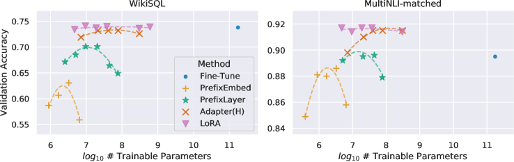
Figure 2: GPT-3 175B validation accuracy vs. number of trainable parameters of several adaptation methods on WikiSQL and MNLI-matched. LoRA exhibits better scalability and task performance. See Section F.2 for more details on the plotted data points.

Transformer Language Models.   Transformer (Vaswani et al., 2017) is a sequence-to-sequence architecture that makes heavy use of self-attention. Radford et al. (a) applied it to autoregressive language modeling by using a stack of Transformer decoders. Since then, Transformer-based language models have dominated NLP, achieving the state-of-the-art in many tasks. A new paradigm emerged with BERT (Devlin et al., 2019b) and GPT-2 (Radford et al., b) – both are large Transformer language models trained on a large amount of text – where fine-tuning on task-specific data after pre-training on general domain data provides a significant performance gain compared to training on task-specific data directly. Training larger Transformers generally results in better performance and remains an active research direction. GPT-3 (Brown et al., 2020) is the largest single Transformer language model trained to-date with 175B parameters.

Prompt Engineering and Fine-Tuning.   While GPT-3 175B can adapt its behavior with just a few additional training examples, the result depends heavily on the input prompt (Brown et al., 2020). This necessitates an empirical art of composing and formatting the prompt to maximize a model’s performance on a desired task, which is known as prompt engineering or prompt hacking. Fine-tuning retrains a model pre-trained on general domains to a specific task Devlin et al. (2019b); Radford et al. (a). Variants of it include learning just a subset of the parameters Devlin et al. (2019b); Collobert & Weston (2008), yet practitioners often retrain all of them to maximize the downstream performance. However, the enormity of GPT-3 175B makes it challenging to perform fine-tuning in the usual way due to the large checkpoint it produces and the high hardware barrier to entry since it has the same memory footprint as pre-training.

Parameter-Efficient Adaptation.   Many have proposed inserting adapter layers between existing layers in a neural network (Houlsby et al., 2019; Rebuffi et al., 2017; Lin et al., 2020). Our method uses a similar bottleneck structure to impose a low-rank constraint on the weight updates. The key functional difference is that our learned weights can be merged with the main weights during inference, thus not introducing any latency, which is not the case for the adapter layers (Section 3). A comtenporary extension of adapter is compacter (Mahabadi et al., 2021), which essentially parametrizes the adapter layers using Kronecker products with some predetermined weight sharing scheme. Similarly, combining LoRA with other tensor product-based methods could potentially improve its parameter efficiency, which we leave to future work. More recently, many proposed optimizing the input word embeddings in lieu of fine-tuning, akin to a continuous and differentiable generalization of prompt engineering (Li & Liang, 2021; Lester et al., 2021; Hambardzumyan et al., 2020; Liu et al., 2021). We include comparisons with Li & Liang (2021) in our experiment section. However, this line of works can only scale up by using more special tokens in the prompt, which take up available sequence length for task tokens when positional embeddings are learned.

Low-Rank Structures in Deep Learning.   Low-rank structure is very common in machine learning. A lot of machine learning problems have certain intrinsic low-rank structure (Li et al., 2016; Cai et al., 2010; Li et al., 2018b; Grasedyck et al., 2013). Moreover, it is known that for many deep learning tasks, especially those with a heavily over-parametrized neural network, the learned neural network will enjoy low-rank properties after training (Oymak et al., 2019). Some prior works even explicitly impose the low-rank constraint when training the original neural network (Sainath et al., 2013; Povey et al., 2018; Zhang et al., 2014; Jaderberg et al., 2014; Zhao et al., 2016; Khodak et al., 2021; Denil et al., 2014); however, to the best of our knowledge, none of these works considers low-rank update to a frozen model for adaptation to downstream tasks. In theory literature, it is known that neural networks outperform other classical learning methods, including the corresponding (finite-width) neural tangent kernels (Allen-Zhu et al., 2019; Li & Liang, 2018) when the underlying concept class has certain low-rank structure (Ghorbani et al., 2020; Allen-Zhu & Li, 2019; 2020a). Another theoretical result in Allen-Zhu & Li (2020b) suggests that low-rank adaptations can be useful for adversarial training. In sum, we believe that our proposed low-rank adaptation update is well-motivated by the literature.

Given the empirical advantage of LoRA, we hope to further explain the properties of the low-rank adaptation learned from downstream tasks. Note that the low-rank structure not only lowers the hardware barrier to entry which allows us to run multiple experiments in parallel, but also gives better interpretability of how the update weights are correlated with the pre-trained weights. We focus our study on GPT-3 175B, where we achieved the largest reduction of trainable parameters (up to 10,000×\times) without adversely affecting task performances.

We perform a sequence of empirical studies to answer the following questions: 1) Given a parameter budget constraint, which subset of weight matrices in a pre-trained Transformer should we adapt to maximize downstream performance? 2) Is the “optimal” adaptation matrix Δ​WΔ𝑊\Delta W really rank-deficient? If so, what is a good rank to use in practice? 3) What is the connection between Δ​WΔ𝑊\Delta W and W𝑊W? Does Δ​WΔ𝑊\Delta W highly correlate with W𝑊W? How large is Δ​WΔ𝑊\Delta W comparing to W𝑊W?

We believe that our answers to question (2) and (3) shed light on the fundamental principles of using pre-trained language models for downstream tasks, which is a critical topic in NLP.

Given a limited parameter budget, which types of weights should we adapt with LoRA to obtain the best performance on downstream tasks? As mentioned in Section 4.2, we only consider weight matrices in the self-attention module. We set a parameter budget of 18M (roughly 35MB if stored in FP16) on GPT-3 175B, which corresponds to r=8𝑟8r=8 if we adapt one type of attention weights or r=4𝑟4r=4 if we adapt two types, for all 96 layers. The result is presented in Table 5.

# of Trainable Parameters = 18M

Weight Type

Wqsubscript𝑊𝑞W_{q}

Wksubscript𝑊𝑘W_{k}

Wvsubscript𝑊𝑣W_{v}

Wosubscript𝑊𝑜W_{o}

Wq,Wksubscript𝑊𝑞subscript𝑊𝑘W_{q},W_{k}

Wq,Wvsubscript𝑊𝑞subscript𝑊𝑣W_{q},W_{v}

Wq,Wk,Wv,Wosubscript𝑊𝑞subscript𝑊𝑘subscript𝑊𝑣subscript𝑊𝑜W_{q},W_{k},W_{v},W_{o}

Rank r𝑟r

8

8

8

8

4

4

2

WikiSQL (±0.5plus-or-minus0.5\pm 0.5%)

70.4

70.0

73.0

73.2

71.4

73.7

73.7

MultiNLI (±0.1plus-or-minus0.1\pm 0.1%)

91.0

90.8

91.0

91.3

91.3

91.3

91.7

Table 5: Validation accuracy on WikiSQL and MultiNLI after applying LoRA to different types of attention weights in GPT-3, given the same number of trainable parameters. Adapting both Wqsubscript𝑊𝑞W_{q} and Wvsubscript𝑊𝑣W_{v} gives the best performance overall. We find the standard deviation across random seeds to be consistent for a given dataset, which we report in the first column.

Note that putting all the parameters in Δ​WqΔsubscript𝑊𝑞\Delta W_{q} or Δ​WkΔsubscript𝑊𝑘\Delta W_{k} results in significantly lower performance, while adapting both Wqsubscript𝑊𝑞W_{q} and Wvsubscript𝑊𝑣W_{v} yields the best result. This suggests that even a rank of four captures enough information in Δ​WΔ𝑊\Delta W such that it is preferable to adapt more weight matrices than adapting a single type of weights with a larger rank.

We turn our attention to the effect of rank r𝑟r on model performance. We adapt {Wq,Wv}subscript𝑊𝑞subscript𝑊𝑣\{W_{q},W_{v}\}, {Wq,Wk,Wv,Wc}subscript𝑊𝑞subscript𝑊𝑘subscript𝑊𝑣subscript𝑊𝑐\{W_{q},W_{k},W_{v},W_{c}\}, and just Wqsubscript𝑊𝑞W_{q} for a comparison.

Weight Type

r=1𝑟1r=1

r=2𝑟2r=2

r=4𝑟4r=4

r=8𝑟8r=8

r=64𝑟64r=64

WikiSQL(±0.5plus-or-minus0.5\pm 0.5%)

Wqsubscript𝑊𝑞W_{q}

68.8

69.6

70.5

70.4

70.0

Wq,Wvsubscript𝑊𝑞subscript𝑊𝑣W_{q},W_{v}

73.4

73.3

73.7

73.8

73.5

Wq,Wk,Wv,Wosubscript𝑊𝑞subscript𝑊𝑘subscript𝑊𝑣subscript𝑊𝑜W_{q},W_{k},W_{v},W_{o}

74.1

73.7

74.0

74.0

73.9

MultiNLI (±0.1plus-or-minus0.1\pm 0.1%)

Wqsubscript𝑊𝑞W_{q}

90.7

90.9

91.1

90.7

90.7

Wq,Wvsubscript𝑊𝑞subscript𝑊𝑣W_{q},W_{v}

91.3

91.4

91.3

91.6

91.4

Wq,Wk,Wv,Wosubscript𝑊𝑞subscript𝑊𝑘subscript𝑊𝑣subscript𝑊𝑜W_{q},W_{k},W_{v},W_{o}

91.2

91.7

91.7

91.5

91.4

Table 6: Validation accuracy on WikiSQL and MultiNLI with different rank r𝑟r. To our surprise, a rank as small as one suffices for adapting both Wqsubscript𝑊𝑞W_{q} and Wvsubscript𝑊𝑣W_{v} on these datasets while training Wqsubscript𝑊𝑞W_{q} alone needs a larger r𝑟r. We conduct a similar experiment on GPT-2 in Section H.2.

Table 6 shows that, surprisingly, LoRA already performs competitively with a very small r𝑟r (more so for {Wq,Wv}subscript𝑊𝑞subscript𝑊𝑣\{W_{q},W_{v}\} than just Wqsubscript𝑊𝑞W_{q}). This suggests the update matrix Δ​WΔ𝑊\Delta W could have a very small “intrinsic rank”. To further support this finding, we check the overlap of the subspaces learned by different choices of r𝑟r and by different random seeds. We argue that increasing r𝑟r does not cover a more meaningful subspace, which suggests that a low-rank adaptation matrix is sufficient.

Subspace similarity between different r𝑟r.   Given Ar=8subscript𝐴𝑟8A_{r=8} and Ar=64subscript𝐴𝑟64A_{r=64} which are the learned adaptation matrices with rank r=8𝑟8r=8 and 646464 using the same pre-trained model, we perform singular value decomposition and obtain the right-singular unitary matrices UAr=8subscript𝑈subscript𝐴𝑟8U_{A_{r=8}} and UAr=64subscript𝑈subscript𝐴𝑟64U_{A_{r=64}}. We hope to answer: how much of the subspace spanned by the top i𝑖i singular vectors in UAr=8subscript𝑈subscript𝐴𝑟8U_{A_{r=8}} (for 1≤i≤81𝑖81\leq i\leq 8) is contained in the subspace spanned by top j𝑗j singular vectors of UAr=64subscript𝑈subscript𝐴𝑟64U_{A_{r=64}} (for 1≤j≤641𝑗641\leq j\leq 64)? We measure this quantity with a normalized subspace similarity based on the Grassmann distance (See Appendix G for a more formal discussion)

ϕ​(Ar=8,Ar=64,i,j)=‖UAr=8i⊤​UAr=64j‖F2min⁡(i,j)∈[0,1]italic-ϕsubscript𝐴𝑟8subscript𝐴𝑟64𝑖𝑗superscriptsubscriptnormsuperscriptsubscript𝑈subscript𝐴𝑟8limit-from𝑖topsuperscriptsubscript𝑈subscript𝐴𝑟64𝑗𝐹2𝑖𝑗01\phi(A_{r=8},A_{r=64},i,j)=\frac{||U_{A_{r=8}}^{i\top}U_{A_{r=64}}^{j}||_{F}^{2}}{\min(i,j)}\in[0,1]

(4)

where UAr=8isuperscriptsubscript𝑈subscript𝐴𝑟8𝑖U_{A_{r=8}}^{i} represents the columns of UAr=8subscript𝑈subscript𝐴𝑟8U_{A_{r=8}} corresponding to the top-i𝑖i singular vectors.

ϕ​(⋅)italic-ϕ⋅\phi(\cdot) has a range of [0,1]01[0,1], where 111 represents a complete overlap of subspaces and 00 a complete separation. See Figure 3 for how ϕitalic-ϕ\phi changes as we vary i𝑖i and j𝑗j. We only look at the 48th layer (out of 96) due to space constraint, but the conclusion holds for other layers as well, as shown in Section H.1.

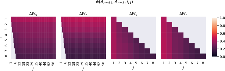
Figure 3: Subspace similarity between column vectors of Ar=8subscript𝐴𝑟8A_{r=8} and Ar=64subscript𝐴𝑟64A_{r=64} for both Δ​WqΔsubscript𝑊𝑞\Delta W_{q} and Δ​WvΔsubscript𝑊𝑣\Delta W_{v}. The third and the fourth figures zoom in on the lower-left triangle in the first two figures. The top directions in r=8𝑟8r=8 are included in r=64𝑟64r=64, and vice versa.

We make an important observation from Figure 3.

Directions corresponding to the top singular vector overlap significantly between Ar=8subscript𝐴𝑟8A_{r=8} and Ar=64subscript𝐴𝑟64A_{r=64}, while others do not. Specifically, Δ​WvΔsubscript𝑊𝑣\Delta W_{v} (resp. Δ​WqΔsubscript𝑊𝑞\Delta W_{q}) of Ar=8subscript𝐴𝑟8A_{r=8} and Δ​WvΔsubscript𝑊𝑣\Delta W_{v} (resp. Δ​WqΔsubscript𝑊𝑞\Delta W_{q}) of Ar=64subscript𝐴𝑟64A_{r=64} share a subspace of dimension 1 with normalized similarity >0.5absent0.5>0.5, providing an explanation of why r=1𝑟1r=1 performs quite well in our downstream tasks for GPT-3.

Since both Ar=8subscript𝐴𝑟8A_{r=8} and Ar=64subscript𝐴𝑟64A_{r=64} are learned using the same pre-trained model, Figure 3 indicates that the top singular-vector directions of Ar=8subscript𝐴𝑟8A_{r=8} and Ar=64subscript𝐴𝑟64A_{r=64} are the most useful, while other directions potentially contain mostly random noises accumulated during training. Hence, the adaptation matrix can indeed have a very low rank.

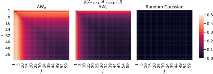
Figure 4: Left and Middle: Normalized subspace similarity between the column vectors of Ar=64subscript𝐴𝑟64A_{r=64} from two random seeds, for both Δ​WqΔsubscript𝑊𝑞\Delta W_{q} and Δ​WvΔsubscript𝑊𝑣\Delta W_{v} in the 48-th layer. Right: the same heat-map between the column vectors of two random Gaussian matrices. See Section H.1 for other layers.

Subspace similarity between different random seeds.   We further confirm this by plotting the normalized subspace similarity between two randomly seeded runs with r=64𝑟64r=64, shown in Figure 4. Δ​WqΔsubscript𝑊𝑞\Delta W_{q} appears to have a higher “intrinsic rank” than Δ​WvΔsubscript𝑊𝑣\Delta W_{v}, since more common singular value directions are learned by both runs for Δ​WqΔsubscript𝑊𝑞\Delta W_{q}, which is in line with our empirical observation in Table 6. As a comparison, we also plot two random Gaussian matrices, which do not share any common singular value directions with each other.

We further investigate the relationship between Δ​WΔ𝑊\Delta W and W𝑊W. In particular, does Δ​WΔ𝑊\Delta W highly correlate with W𝑊W? (Or mathematically, is Δ​WΔ𝑊\Delta W mostly contained in the top singular directions of W𝑊W?) Also, how “large” is Δ​WΔ𝑊\Delta W comparing to its corresponding directions in W𝑊W? This can shed light on the underlying mechanism for adapting pre-trained language models.

To answer these questions, we project W𝑊W onto the r𝑟r-dimensional subspace of Δ​WΔ𝑊\Delta W by computing U⊤​W​V⊤superscript𝑈top𝑊superscript𝑉topU^{\top}WV^{\top}, with U𝑈U/V𝑉V being the left/right singular-vector matrix of Δ​WΔ𝑊\Delta W. Then, we compare the Frobenius norm between ‖U⊤​W​V⊤‖Fsubscriptnormsuperscript𝑈top𝑊superscript𝑉top𝐹\|U^{\top}WV^{\top}\|_{F} and ‖W‖Fsubscriptnorm𝑊𝐹\|W\|_{F}. As a comparison, we also compute ‖U⊤​W​V⊤‖Fsubscriptnormsuperscript𝑈top𝑊superscript𝑉top𝐹\|U^{\top}WV^{\top}\|_{F} by replacing U,V𝑈𝑉U,V with the top r𝑟r singular vectors of W𝑊W or a random matrix.

r=4𝑟4r=4

r=64𝑟64r=64

Δ​WqΔsubscript𝑊𝑞\Delta W_{q}

Wqsubscript𝑊𝑞W_{q}

Random

Δ​WqΔsubscript𝑊𝑞\Delta W_{q}

Wqsubscript𝑊𝑞W_{q}

Random

‖U⊤​Wq​V⊤‖F=subscriptnormsuperscript𝑈topsubscript𝑊𝑞superscript𝑉top𝐹absent||U^{\top}W_{q}V^{\top}||_{F}=

0.32

21.67

0.02

1.90

37.71

0.33

‖Wq‖F=61.95subscriptnormsubscript𝑊𝑞𝐹61.95||W_{q}||_{F}=61.95

‖Δ​Wq‖F=6.91subscriptnormΔsubscript𝑊𝑞𝐹6.91||\Delta W_{q}||_{F}=6.91

‖Δ​Wq‖F=3.57subscriptnormΔsubscript𝑊𝑞𝐹3.57||\Delta W_{q}||_{F}=3.57

Table 7: The Frobenius norm of U⊤​Wq​V⊤superscript𝑈topsubscript𝑊𝑞superscript𝑉topU^{\top}W_{q}V^{\top} where U𝑈U and V𝑉V are the left/right top r𝑟r singular vector directions of either (1) Δ​WqΔsubscript𝑊𝑞\Delta W_{q}, (2) Wqsubscript𝑊𝑞W_{q}, or (3) a random matrix. The weight matrices are taken from the 48th layer of GPT-3.

We draw several conclusions from Table 7. First, Δ​WΔ𝑊\Delta W has a stronger correlation with W𝑊W compared to a random matrix, indicating that Δ​WΔ𝑊\Delta W amplifies some features that are already in W𝑊W. Second, instead of repeating the top singular directions of W𝑊W, Δ​WΔ𝑊\Delta W only amplifies directions that are not emphasized in W𝑊W. Third, the amplification factor is rather huge: 21.5≈6.91/0.3221.56.910.3221.5\approx 6.91/0.32 for r=4𝑟4r=4. See Section H.4 for why r=64𝑟64r=64 has a smaller amplification factor. We also provide a visualization in Section H.3 for how the correlation changes as we include more top singular directions from Wqsubscript𝑊𝑞W_{q}. This suggests that the low-rank adaptation matrix potentially amplifies the important features for specific downstream tasks that were learned but not emphasized in the general pre-training model.

Fine-tuning enormous language models is prohibitively expensive in terms of the hardware required and the storage/switching cost for hosting independent instances for different tasks. We propose LoRA, an efficient adaptation strategy that neither introduces inference latency nor reduces input sequence length while retaining high model quality. Importantly, it allows for quick task-switching when deployed as a service by sharing the vast majority of the model parameters. While we focused on Transformer language models, the proposed principles are generally applicable to any neural networks with dense layers.

There are many directions for future works. 1) LoRA can be combined with other efficient adaptation methods, potentially providing orthogonal improvement. 2) The mechanism behind fine-tuning or LoRA is far from clear – how are features learned during pre-training transformed to do well on downstream tasks? We believe that LoRA makes it more tractable to answer this than full fine-tuning. 3) We mostly depend on heuristics to select the weight matrices to apply LoRA to. Are there more principled ways to do it? 4) Finally, the rank-deficiency of Δ​WΔ𝑊\Delta W suggests that W𝑊W could be rank-deficient as well, which can also be a source of inspiration for future works.

• Aghajanyan et al. (2020) Armen Aghajanyan, Luke Zettlemoyer, and Sonal Gupta. Intrinsic Dimensionality Explains the Effectiveness of Language Model Fine-Tuning. arXiv:2012.13255 [cs], December 2020. URL http://arxiv.org/abs/2012.13255.
• Allen-Zhu & Li (2019) Zeyuan Allen-Zhu and Yuanzhi Li. What Can ResNet Learn Efficiently, Going Beyond Kernels? In NeurIPS, 2019. Full version available at http://arxiv.org/abs/1905.10337.
• Allen-Zhu & Li (2020a) Zeyuan Allen-Zhu and Yuanzhi Li. Backward feature correction: How deep learning performs deep learning. arXiv preprint arXiv:2001.04413, 2020a.
• Allen-Zhu & Li (2020b) Zeyuan Allen-Zhu and Yuanzhi Li. Feature purification: How adversarial training performs robust deep learning. arXiv preprint arXiv:2005.10190, 2020b.
• Allen-Zhu et al. (2019) Zeyuan Allen-Zhu, Yuanzhi Li, and Zhao Song. A convergence theory for deep learning via over-parameterization. In ICML, 2019. Full version available at http://arxiv.org/abs/1811.03962.
• Ba et al. (2016) Jimmy Lei Ba, Jamie Ryan Kiros, and Geoffrey E. Hinton. Layer normalization, 2016.
• Brown et al. (2020) Tom B. Brown, Benjamin Mann, Nick Ryder, Melanie Subbiah, Jared Kaplan, Prafulla Dhariwal, Arvind Neelakantan, Pranav Shyam, Girish Sastry, Amanda Askell, Sandhini Agarwal, Ariel Herbert-Voss, Gretchen Krueger, Tom Henighan, Rewon Child, Aditya Ramesh, Daniel M. Ziegler, Jeffrey Wu, Clemens Winter, Christopher Hesse, Mark Chen, Eric Sigler, Mateusz Litwin, Scott Gray, Benjamin Chess, Jack Clark, Christopher Berner, Sam McCandlish, Alec Radford, Ilya Sutskever, and Dario Amodei. Language Models are Few-Shot Learners. arXiv:2005.14165 [cs], July 2020. URL http://arxiv.org/abs/2005.14165.
• Cai et al. (2010) Jian-Feng Cai, Emmanuel J Candès, and Zuowei Shen. A singular value thresholding algorithm for matrix completion. SIAM Journal on optimization, 20(4):1956–1982, 2010.
• Cer et al. (2017) Daniel Cer, Mona Diab, Eneko Agirre, Inigo Lopez-Gazpio, and Lucia Specia. Semeval-2017 task 1: Semantic textual similarity multilingual and crosslingual focused evaluation. Proceedings of the 11th International Workshop on Semantic Evaluation (SemEval-2017), 2017. doi: 10.18653/v1/s17-2001. URL http://dx.doi.org/10.18653/v1/S17-2001.
• Collobert & Weston (2008) Ronan Collobert and Jason Weston. A unified architecture for natural language processing: deep neural networks with multitask learning. In Proceedings of the 25th international conference on Machine learning, ICML ’08, pp.  160–167, New York, NY, USA, July 2008. Association for Computing Machinery. ISBN 978-1-60558-205-4. doi: 10.1145/1390156.1390177. URL https://doi.org/10.1145/1390156.1390177.
• Denil et al. (2014) Misha Denil, Babak Shakibi, Laurent Dinh, Marc’Aurelio Ranzato, and Nando de Freitas. Predicting parameters in deep learning, 2014.
• Devlin et al. (2019a) Jacob Devlin, Ming-Wei Chang, Kenton Lee, and Kristina Toutanova. Bert: Pre-training of deep bidirectional transformers for language understanding, 2019a.
• Devlin et al. (2019b) Jacob Devlin, Ming-Wei Chang, Kenton Lee, and Kristina Toutanova. BERT: Pre-training of Deep Bidirectional Transformers for Language Understanding. arXiv:1810.04805 [cs], May 2019b. URL http://arxiv.org/abs/1810.04805. arXiv: 1810.04805.
• Dolan & Brockett (2005) William B. Dolan and Chris Brockett. Automatically constructing a corpus of sentential paraphrases. In Proceedings of the Third International Workshop on Paraphrasing (IWP2005), 2005. URL https://aclanthology.org/I05-5002.
• Gardent et al. (2017) Claire Gardent, Anastasia Shimorina, Shashi Narayan, and Laura Perez-Beltrachini. The webnlg challenge: Generating text from rdf data. In Proceedings of the 10th International Conference on Natural Language Generation, pp.  124–133, 2017.
• Ghorbani et al. (2020) Behrooz Ghorbani, Song Mei, Theodor Misiakiewicz, and Andrea Montanari. When do neural networks outperform kernel methods? arXiv preprint arXiv:2006.13409, 2020.
• Gliwa et al. (2019) Bogdan Gliwa, Iwona Mochol, Maciej Biesek, and Aleksander Wawer. Samsum corpus: A human-annotated dialogue dataset for abstractive summarization. CoRR, abs/1911.12237, 2019. URL http://arxiv.org/abs/1911.12237.
• Grasedyck et al. (2013) Lars Grasedyck, Daniel Kressner, and Christine Tobler. A literature survey of low-rank tensor approximation techniques. GAMM-Mitteilungen, 36(1):53–78, 2013.
• Ham & Lee (2008) Jihun Ham and Daniel D. Lee. Grassmann discriminant analysis: a unifying view on subspace-based learning. In ICML, pp.  376–383, 2008. URL https://doi.org/10.1145/1390156.1390204.
• Hambardzumyan et al. (2020) Karen Hambardzumyan, Hrant Khachatrian, and Jonathan May. WARP: Word-level Adversarial ReProgramming. arXiv:2101.00121 [cs], December 2020. URL http://arxiv.org/abs/2101.00121. arXiv: 2101.00121.
• He et al. (2021) Pengcheng He, Xiaodong Liu, Jianfeng Gao, and Weizhu Chen. Deberta: Decoding-enhanced bert with disentangled attention, 2021.
• Houlsby et al. (2019) Neil Houlsby, Andrei Giurgiu, Stanislaw Jastrzebski, Bruna Morrone, Quentin de Laroussilhe, Andrea Gesmundo, Mona Attariyan, and Sylvain Gelly. Parameter-Efficient Transfer Learning for NLP. arXiv:1902.00751 [cs, stat], June 2019. URL http://arxiv.org/abs/1902.00751.
• Jaderberg et al. (2014) Max Jaderberg, Andrea Vedaldi, and Andrew Zisserman. Speeding up convolutional neural networks with low rank expansions. arXiv preprint arXiv:1405.3866, 2014.
• Khodak et al. (2021) Mikhail Khodak, Neil Tenenholtz, Lester Mackey, and Nicolò Fusi. Initialization and regularization of factorized neural layers, 2021.
• Kingma & Ba (2017) Diederik P. Kingma and Jimmy Ba. Adam: A method for stochastic optimization, 2017.
• Lepikhin et al. (2020) Dmitry Lepikhin, HyoukJoong Lee, Yuanzhong Xu, Dehao Chen, Orhan Firat, Yanping Huang, Maxim Krikun, Noam Shazeer, and Zhifeng Chen. Gshard: Scaling giant models with conditional computation and automatic sharding, 2020.
• Lester et al. (2021) Brian Lester, Rami Al-Rfou, and Noah Constant. The Power of Scale for Parameter-Efficient Prompt Tuning. arXiv:2104.08691 [cs], April 2021. URL http://arxiv.org/abs/2104.08691. arXiv: 2104.08691.
• Li et al. (2018a) Chunyuan Li, Heerad Farkhoor, Rosanne Liu, and Jason Yosinski. Measuring the Intrinsic Dimension of Objective Landscapes. arXiv:1804.08838 [cs, stat], April 2018a. URL http://arxiv.org/abs/1804.08838. arXiv: 1804.08838.
• Li & Liang (2021) Xiang Lisa Li and Percy Liang. Prefix-Tuning: Optimizing Continuous Prompts for Generation. arXiv:2101.00190 [cs], January 2021. URL http://arxiv.org/abs/2101.00190.
• Li & Liang (2018) Yuanzhi Li and Yingyu Liang. Learning overparameterized neural networks via stochastic gradient descent on structured data. In Advances in Neural Information Processing Systems, 2018.
• Li et al. (2016) Yuanzhi Li, Yingyu Liang, and Andrej Risteski. Recovery guarantee of weighted low-rank approximation via alternating minimization. In International Conference on Machine Learning, pp. 2358–2367. PMLR, 2016.
• Li et al. (2018b) Yuanzhi Li, Tengyu Ma, and Hongyang Zhang. Algorithmic regularization in over-parameterized matrix sensing and neural networks with quadratic activations. In Conference On Learning Theory, pp.  2–47. PMLR, 2018b.
• Lin et al. (2020) Zhaojiang Lin, Andrea Madotto, and Pascale Fung. Exploring versatile generative language model via parameter-efficient transfer learning. In Findings of the Association for Computational Linguistics: EMNLP 2020, pp.  441–459, Online, November 2020. Association for Computational Linguistics. doi: 10.18653/v1/2020.findings-emnlp.41. URL https://aclanthology.org/2020.findings-emnlp.41.
• Liu et al. (2021) Xiao Liu, Yanan Zheng, Zhengxiao Du, Ming Ding, Yujie Qian, Zhilin Yang, and Jie Tang. GPT Understands, Too. arXiv:2103.10385 [cs], March 2021. URL http://arxiv.org/abs/2103.10385. arXiv: 2103.10385.
• Liu et al. (2019) Yinhan Liu, Myle Ott, Naman Goyal, Jingfei Du, Mandar Joshi, Danqi Chen, Omer Levy, Mike Lewis, Luke Zettlemoyer, and Veselin Stoyanov. Roberta: A robustly optimized bert pretraining approach, 2019.
• Loshchilov & Hutter (2017) Ilya Loshchilov and Frank Hutter. Decoupled weight decay regularization. arXiv preprint arXiv:1711.05101, 2017.
• Loshchilov & Hutter (2019) Ilya Loshchilov and Frank Hutter. Decoupled weight decay regularization, 2019.
• Mahabadi et al. (2021) Rabeeh Karimi Mahabadi, James Henderson, and Sebastian Ruder. Compacter: Efficient low-rank hypercomplex adapter layers, 2021.
• Nan et al. (2020) Linyong Nan, Dragomir Radev, Rui Zhang, Amrit Rau, Abhinand Sivaprasad, Chiachun Hsieh, Xiangru Tang, Aadit Vyas, Neha Verma, Pranav Krishna, et al. Dart: Open-domain structured data record to text generation. arXiv preprint arXiv:2007.02871, 2020.
• Novikova et al. (2017) Jekaterina Novikova, Ondřej Dušek, and Verena Rieser. The e2e dataset: New challenges for end-to-end generation. arXiv preprint arXiv:1706.09254, 2017.
• Oymak et al. (2019) Samet Oymak, Zalan Fabian, Mingchen Li, and Mahdi Soltanolkotabi. Generalization guarantees for neural networks via harnessing the low-rank structure of the jacobian. arXiv preprint arXiv:1906.05392, 2019.
• Pfeiffer et al. (2021) Jonas Pfeiffer, Aishwarya Kamath, Andreas Rücklé, Kyunghyun Cho, and Iryna Gurevych. Adapterfusion: Non-destructive task composition for transfer learning, 2021.
• Povey et al. (2018) Daniel Povey, Gaofeng Cheng, Yiming Wang, Ke Li, Hainan Xu, Mahsa Yarmohammadi, and Sanjeev Khudanpur. Semi-orthogonal low-rank matrix factorization for deep neural networks. In Interspeech, pp.  3743–3747, 2018.
• Radford et al. (a) Alec Radford, Karthik Narasimhan, Tim Salimans, and Ilya Sutskever. Improving Language Understanding by Generative Pre-Training. pp.  12, a.
• Radford et al. (b) Alec Radford, Jeffrey Wu, Rewon Child, David Luan, Dario Amodei, and Ilya Sutskever. Language Models are Unsupervised Multitask Learners. pp.  24, b.
• Rajpurkar et al. (2018) Pranav Rajpurkar, Robin Jia, and Percy Liang. Know what you don’t know: Unanswerable questions for squad. CoRR, abs/1806.03822, 2018. URL http://arxiv.org/abs/1806.03822.
• Rebuffi et al. (2017) Sylvestre-Alvise Rebuffi, Hakan Bilen, and Andrea Vedaldi. Learning multiple visual domains with residual adapters. arXiv:1705.08045 [cs, stat], November 2017. URL http://arxiv.org/abs/1705.08045. arXiv: 1705.08045.
• Rücklé et al. (2020) Andreas Rücklé, Gregor Geigle, Max Glockner, Tilman Beck, Jonas Pfeiffer, Nils Reimers, and Iryna Gurevych. Adapterdrop: On the efficiency of adapters in transformers, 2020.
• Sainath et al. (2013) Tara N Sainath, Brian Kingsbury, Vikas Sindhwani, Ebru Arisoy, and Bhuvana Ramabhadran. Low-rank matrix factorization for deep neural network training with high-dimensional output targets. In 2013 IEEE international conference on acoustics, speech and signal processing, pp.  6655–6659. IEEE, 2013.
• Shoeybi et al. (2020) Mohammad Shoeybi, Mostofa Patwary, Raul Puri, Patrick LeGresley, Jared Casper, and Bryan Catanzaro. Megatron-lm: Training multi-billion parameter language models using model parallelism, 2020.
• Socher et al. (2013) Richard Socher, Alex Perelygin, Jean Wu, Jason Chuang, Christopher D. Manning, Andrew Ng, and Christopher Potts. Recursive deep models for semantic compositionality over a sentiment treebank. In Proceedings of the 2013 Conference on Empirical Methods in Natural Language Processing, pp.  1631–1642, Seattle, Washington, USA, October 2013. Association for Computational Linguistics. URL https://aclanthology.org/D13-1170.
• Vaswani et al. (2017) Ashish Vaswani, Noam Shazeer, Niki Parmar, Jakob Uszkoreit, Llion Jones, Aidan N Gomez, Łukasz Kaiser, and Illia Polosukhin. Attention is all you need. In Proceedings of the 31st International Conference on Neural Information Processing Systems, pp.  6000–6010, 2017.
• Wang et al. (2019) Alex Wang, Amanpreet Singh, Julian Michael, Felix Hill, Omer Levy, and Samuel R. Bowman. Glue: A multi-task benchmark and analysis platform for natural language understanding, 2019.
• Wang et al. (2020) Alex Wang, Yada Pruksachatkun, Nikita Nangia, Amanpreet Singh, Julian Michael, Felix Hill, Omer Levy, and Samuel R. Bowman. Superglue: A stickier benchmark for general-purpose language understanding systems, 2020.
• Warstadt et al. (2018) Alex Warstadt, Amanpreet Singh, and Samuel R Bowman. Neural network acceptability judgments. arXiv preprint arXiv:1805.12471, 2018.
• Williams et al. (2018) Adina Williams, Nikita Nangia, and Samuel Bowman. A broad-coverage challenge corpus for sentence understanding through inference. In Proceedings of the 2018 Conference of the North American Chapter of the Association for Computational Linguistics: Human Language Technologies, Volume 1 (Long Papers), pp.  1112–1122, New Orleans, Louisiana, June 2018. Association for Computational Linguistics. doi: 10.18653/v1/N18-1101. URL https://www.aclweb.org/anthology/N18-1101.
• Wolf et al. (2020) Thomas Wolf, Lysandre Debut, Victor Sanh, Julien Chaumond, Clement Delangue, Anthony Moi, Pierric Cistac, Tim Rault, Rémi Louf, Morgan Funtowicz, Joe Davison, Sam Shleifer, Patrick von Platen, Clara Ma, Yacine Jernite, Julien Plu, Canwen Xu, Teven Le Scao, Sylvain Gugger, Mariama Drame, Quentin Lhoest, and Alexander M. Rush. Transformers: State-of-the-art natural language processing. In Proceedings of the 2020 Conference on Empirical Methods in Natural Language Processing: System Demonstrations, pp.  38–45, Online, October 2020. Association for Computational Linguistics. URL https://www.aclweb.org/anthology/2020.emnlp-demos.6.
• Yang & Hu (2021) Greg Yang and Edward J. Hu. Feature Learning in Infinite-Width Neural Networks. arXiv:2011.14522 [cond-mat], May 2021. URL http://arxiv.org/abs/2011.14522. arXiv: 2011.14522.
• Zaken et al. (2021) Elad Ben Zaken, Shauli Ravfogel, and Yoav Goldberg. Bitfit: Simple parameter-efficient fine-tuning for transformer-based masked language-models, 2021.
• Zhang et al. (2014) Yu Zhang, Ekapol Chuangsuwanich, and James Glass. Extracting deep neural network bottleneck features using low-rank matrix factorization. In 2014 IEEE international conference on acoustics, speech and signal processing (ICASSP), pp.  185–189. IEEE, 2014.
• Zhao et al. (2016) Yong Zhao, Jinyu Li, and Yifan Gong. Low-rank plus diagonal adaptation for deep neural networks. In 2016 IEEE International Conference on Acoustics, Speech and Signal Processing (ICASSP), pp.  5005–5009. IEEE, 2016.
• Zhong et al. (2017) Victor Zhong, Caiming Xiong, and Richard Socher. Seq2sql: Generating structured queries from natural language using reinforcement learning. CoRR, abs/1709.00103, 2017. URL http://arxiv.org/abs/1709.00103.

Few-shot learning, or prompt engineering, is very advantageous when we only have a handful of training samples. However, in practice, we can often afford to curate a few thousand or more training examples for performance-sensitive applications. As shown in Table 8, fine-tuning improves the model performance drastically compared to few-shot learning on datasets large and small. We take the GPT-3 few-shot result on RTE from the GPT-3 paper (Brown et al., 2020). For MNLI-matched, we use two demonstrations per class and six in-context examples in total.

Method

MNLI-m (Val. Acc./%)

RTE (Val. Acc./%)

GPT-3 Few-Shot

40.6

69.0

GPT-3 Fine-Tuned

89.5

85.4

Table 8: Fine-tuning significantly outperforms few-shot learning on GPT-3 (Brown et al., 2020).

Adapter layers are external modules added to a pre-trained model in a sequential manner, whereas our proposal, LoRA, can be seen as external modules added in a parallel manner. Consequently, adapter layers must be computed in addition to the base model, inevitably introducing additional latency. While as pointed out in Rücklé et al. (2020), the latency introduced by adapter layers can be mitigated when the model batch size and/or sequence length is large enough to full utilize the hardware parallelism. We confirm their observation with a similar latency study on GPT-2 medium and point out that there are scenarios, notably online inference where the batch size is small, where the added latency can be significant.

We measure the latency of a single forward pass on an NVIDIA Quadro RTX8000 by averaging over 100 trials. We vary the input batch size, sequence length, and the adapter bottleneck dimension r𝑟r. We test two adapter designs: the original one by Houlsby et al. (2019), which we call AdapterHsuperscriptAdapterH\text{Adapter}^{\text{H}}, and a recent, more efficient variant by Lin et al. (2020), which we call AdapterLsuperscriptAdapterL\text{Adapter}^{\text{L}}. See Section 5.1 for more details on the designs. We plot the slow-down in percentage compared to the no-adapter baseline in Figure 5.

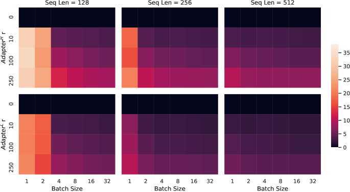
Figure 5: Percentage slow-down of inference latency compared to the no-adapter (r=0𝑟0r=0) baseline. The top row shows the result for AdapterHsuperscriptAdapterH\text{Adapter}^{\text{H}} and the bottom row AdapterLsuperscriptAdapterL\text{Adapter}^{\text{L}}. Larger batch size and sequence length help to mitigate the latency, but the slow-down can be as high as over 30% in an online, short-sequence-length scenario. We tweak the colormap for better visibility.

GLUE Benchmark is a wide-ranging collection of natural language understanding tasks. It includes MNLI (inference, Williams et al. (2018)), SST-2 (sentiment analysis, Socher et al. (2013)), MRPC (paraphrase detection, Dolan & Brockett (2005)), CoLA (linguistic acceptability, Warstadt et al. (2018)), QNLI (inference, Rajpurkar et al. (2018)), QQP (question-answering), RTE (inference), and STS-B (textual similarity, Cer et al. (2017)). The broad coverage makes GLUE benchmark a standard metric to evaluate NLU models such as RoBERTa and DeBERTa. The individual datasets are released under different permissive licenses.

WikiSQL is introduced in  Zhong et al. (2017) and contains 56,3555635556,355/8,42184218,421 training/validation examples. The task is to generate SQL queries from natural language questions and table schemata. We encode context as x={table schema,query}𝑥table schemaqueryx=\{\text{table schema},\text{query}\} and target as y={SQL}𝑦SQLy=\{\text{SQL}\}. The dataset is release under the BSD 3-Clause License.

SAMSum is introduced in  Gliwa et al. (2019) and contains 14,7321473214,732/819819819 training/test examples. It consists of staged chat conversations between two people and corresponding abstractive summaries written by linguists. We encode context as ”\n” concatenated utterances followed by a ”\n\n”, and target as y={summary}𝑦summaryy=\{\text{summary}\}. The dataset is released under the non-commercial licence: Creative Commons BY-NC-ND 4.0.

E2E NLG Challenge was first introduced in  Novikova et al. (2017) as a dataset for training end-to-end, data-driven natural language generation systems and is commonly used for data-to-text evaluation. The E2E dataset consists of roughly 42,0004200042,000 training, 4,60046004,600 validation, and 4,60046004,600 test examples from the restaurant domain. Each source table used as input can have multiple references. Each sample input (x,y)𝑥𝑦(x,y) consists of a sequence of slot-value pairs, along with a corresponding natural language reference text. The dataset is released under Creative Commons BY-NC-SA 4.0.

DART is an open-domain data-to-text dataset described in Nan et al. (2020). DART inputs are structured as sequences of ENTITY — RELATION — ENTITY triples. With 82​K82𝐾~{}82K examples in total, DART is a significantly larger and more complex data-to-text task compared to E2E. The dataset is released under the MIT license.

WebNLG is another commonly used dataset for data-to-text evaluation (Gardent et al., 2017). With 22​K22𝐾~{}22K examples in total WebNLG comprises 14 distinct categories, nine of which are seen during training. Since five of the 14 total categories are not seen during training, but are represented in the test set, evaluation is typically broken out by “seen” categories (S), “unseen” categories (U) and “all” (A). Each input example is represented by a sequence of SUBJECT — PROPERTY — OBJECT triples. The dataset is released under Creative Commons BY-NC-SA 4.0.

We train using AdamW with a linear learning rate decay schedule. We sweep learning rate, number of training epochs, and batch size for LoRA. Following Liu et al. (2019), we initialize the LoRA modules to our best MNLI checkpoint when adapting to MRPC, RTE, and STS-B, instead of the usual initialization; the pre-trained model stays frozen for all tasks. We report the median over 5 random seeds; the result for each run is taken from the best epoch. For a fair comparison with the setup in Houlsby et al. (2019) and Pfeiffer et al. (2021), we restrict the model sequence length to 128 and used a fixed batch size for all tasks. Importantly, we start with the pre-trained RoBERTa large model when adapting to MRPC, RTE, and STS-B, instead of a model already adapted to MNLI. The runs with this restricted setup are marked with ††\dagger. See the hyperparameters used in our runs in Table 9.

Method

Dataset

MNLI

SST-2

MRPC

CoLA

QNLI

QQP

RTE

STS-B

Optimizer

AdamW

Warmup Ratio

0.06

LR Schedule

Linear

RoBERTa base LoRA

Batch Size

16

16

16

32

32

16

32

16

# Epochs

30

60

30

80

25

25

80

40

Learning Rate

5E-04

5E-04

4E-04

4E-04

4E-04

5E-04

5E-04

4E-04

LoRA Config.

rq=rv=8subscript𝑟𝑞subscript𝑟𝑣8r_{q}=r_{v}=8

LoRA α𝛼\alpha

8

Max Seq. Len.

512

RoBERTa large LoRA

Batch Size

4

4

4

4

4

4

8

8

# Epochs

10

10

20

20

10

20

20

30

Learning Rate

3E-04

4E-04

3E-04

2E-04

2E-04

3E-04

4E-04

2E-04

LoRA Config.

rq=rv=8subscript𝑟𝑞subscript𝑟𝑣8r_{q}=r_{v}=8

LoRA α𝛼\alpha

16

Max Seq. Len.

128

128

512

128

512

512

512

512

RoBERTa large LoRA††\dagger

Batch Size

4

# Epochs

10

10

20

20

10

20

20

10

Learning Rate

3E-04

4E-04

3E-04

2E-04

2E-04

3E-04

4E-04

2E-04

LoRA Config.

rq=rv=8subscript𝑟𝑞subscript𝑟𝑣8r_{q}=r_{v}=8

LoRA α𝛼\alpha

16

Max Seq. Len.

128

RoBERTa large AdptPsuperscriptAdptP\text{Adpt}^{\text{P}} (3M)††\dagger

Batch Size

32

# Epochs

10

20

20

20

10

20

20

20

Learning Rate

3E-05

3E-05

3E-04

3E-04

3E-04

3E-04

3E-04

3E-04

Bottleneck r𝑟r

64

Max Seq. Len.

128

RoBERTa large AdptPsuperscriptAdptP\text{Adpt}^{\text{P}} (0.8M)††\dagger

Batch Size

32

# Epochs

5

20

20

20

10

20

20

20

Learning Rate

3E-04

3E-04

3E-04

3E-04

3E-04

3E-04

3E-04

3E-04

Bottleneck r𝑟r

16

Max Seq. Len.

128

RoBERTa large AdptHsuperscriptAdptH\text{Adpt}^{\text{H}} (6M)††\dagger

Batch Size

32

# Epochs

10

5

10

10

5

20

20

10

Learning Rate

3E-05

3E-04

3E-04

3E-04

3E-04

3E-04

3E-04

3E-04

Bottleneck r𝑟r

64

Max Seq. Len.

128

RoBERTa large AdptHsuperscriptAdptH\text{Adpt}^{\text{H}} (0.8M)††\dagger

Batch Size

32

# Epochs

10

5

10

10

5

20

20

10

Learning Rate

3E-04

3E-04

3E-04

3E-04

3E-04

3E-04

3E-04

3E-04

Bottleneck r𝑟r

8

Max Seq. Len.

128

Table 9: The hyperparameters we used for RoBERTa on the GLUE benchmark.

We again train using AdamW with a linear learning rate decay schedule. Following He et al. (2021), we tune learning rate, dropout probability, warm-up steps, and batch size. We use the same model sequence length used by (He et al., 2021) to keep our comparison fair. Following He et al. (2021), we initialize the LoRA modules to our best MNLI checkpoint when adapting to MRPC, RTE, and STS-B, instead of the usual initialization; the pre-trained model stays frozen for all tasks. We report the median over 5 random seeds; the result for each run is taken from the best epoch. See the hyperparameters used in our runs in Table 10.

Method

Dataset

MNLI

SST-2

MRPC

CoLA

QNLI

QQP

RTE

STS-B

Optimizer

AdamW

Warmup Ratio

0.1

LR Schedule

Linear

DeBERTa XXL LoRA

Batch Size

8

8

32

4

6

8

4

4

# Epochs

5

16

30

10

8

11

11

10

Learning Rate

1E-04

6E-05

2E-04

1E-04

1E-04

1E-04

2E-04

2E-04

Weight Decay

0

0.01

0.01

0

0.01

0.01

0.01

0.1

CLS Dropout

0.15

0

0

0.1

0.1

0.2

0.2

0.2

LoRA Config.

rq=rv=8subscript𝑟𝑞subscript𝑟𝑣8r_{q}=r_{v}=8

LoRA α𝛼\alpha

8

Max Seq. Len.

256

128

128

64

512

320

320

128

Table 10: The hyperparameters for DeBERTa XXL on tasks included in the GLUE benchmark.

We train all of our GPT-2 models using AdamW (Loshchilov & Hutter, 2017) with a linear learning rate schedule for 5 epochs. We use the batch size, learning rate, and beam search beam size described in Li & Liang (2021). Accordingly, we also tune the above hyperparameters for LoRA. We report the mean over 3 random seeds; the result for each run is taken from the best epoch. The hyperparameters used for LoRA in GPT-2 are listed in Table 11. For those used for other baselines, see Li & Liang (2021).

Dataset

E2E

WebNLG

DART

Training

Optimizer

AdamW

Weight Decay

0.01

0.01

0.0

Dropout Prob

0.1

0.1

0.0

Batch Size

8

# Epoch

5

Warmup Steps

500

Learning Rate Schedule

Linear

Label Smooth

0.1

0.1

0.0

Learning Rate

0.0002

Adaptation

rq=rv=4subscript𝑟𝑞subscript𝑟𝑣4r_{q}=r_{v}=4

LoRA α𝛼\alpha

32

Inference

Beam Size

10

Length Penalty

0.9

0.8

0.8

no repeat ngram size

4

Table 11: The hyperparameters for GPT-2 LoRA on E2E, WebNLG and DART.

For all GPT-3 experiments, we train using AdamW (Loshchilov & Hutter, 2017) for 2 epochs with a batch size of 128 samples and a weight decay factor of 0.1. We use a sequence length of 384 for WikiSQL (Zhong et al., 2017), 768 for MNLI (Williams et al., 2018), and 2048 for SAMSum (Gliwa et al., 2019). We tune learning rate for all method-dataset combinations. See Section D.4 for more details on the hyperparameters used. For prefix-embedding tuning, we find the optimal lpsubscript𝑙𝑝l_{p} and lisubscript𝑙𝑖l_{i} to be 256 and 8, respectively, totalling 3.2​M3.2𝑀3.2M trainable parameters. We use lp=8subscript𝑙𝑝8l_{p}=8 and li=8subscript𝑙𝑖8l_{i}=8 for prefix-layer tuning with 20.2​M20.2𝑀20.2M trainable parameters to obtain the overall best performance. We present two parameter budgets for LoRA: 4.7M (rq=rv=1subscript𝑟𝑞subscript𝑟𝑣1r_{q}=r_{v}=1 or rv=2subscript𝑟𝑣2r_{v}=2) and 37.7M (rq=rv=8subscript𝑟𝑞subscript𝑟𝑣8r_{q}=r_{v}=8 or rq=rk=rv=ro=2subscript𝑟𝑞subscript𝑟𝑘subscript𝑟𝑣subscript𝑟𝑜2r_{q}=r_{k}=r_{v}=r_{o}=2). We report the best validation performance from each run. The training hyperparameters used in our GPT-3 experiments are listed in Table 12.

Hyperparameters

Fine-Tune

PreEmbed

PreLayer

BitFit

AdapterHsuperscriptAdapterH\text{Adapter}^{\text{H}}

LoRA

Optimizer

AdamW

Batch Size

128

# Epoch

2

Warmup Tokens

250,000

LR Schedule

Linear

Learning Rate

5.00E-06

5.00E-04

1.00E-04

1.6E-03

1.00E-04

2.00E-04

Table 12: The training hyperparameters used for different GPT-3 adaption methods. We use the same hyperparameters for all datasets after tuning learning rate.

LoRA can be naturally combined with existing prefix-based approaches. In this section, we evaluate two combinations of LoRA and variants of prefix-tuning on WikiSQL and MNLI.

LoRA+PrefixEmbed (LoRA+PE) combines LoRA with prefix-embedding tuning, where we insert lp+lisubscript𝑙𝑝subscript𝑙𝑖l_{p}+l_{i} special tokens whose embeddings are treated as trainable parameters. For more on prefix-embedding tuning, see Section 5.1.

LoRA+PrefixLayer (LoRA+PL) combines LoRA with prefix-layer tuning. We also insert lp+lisubscript𝑙𝑝subscript𝑙𝑖l_{p}+l_{i} special tokens; however, instead of letting the hidden representations of these tokens evolve naturally, we replace them after every Transformer block with an input agnostic vector. Thus, both the embeddings and subsequent Transformer block activations are treated as trainable parameters. For more on prefix-layer tuning, see Section 5.1.

In Table 15, we show the evaluation results of LoRA+PE and LoRA+PL on WikiSQL and MultiNLI. First of all, LoRA+PE significantly outperforms both LoRA and prefix-embedding tuning on WikiSQL, which indicates that LoRA is somewhat orthogonal to prefix-embedding tuning. On MultiNLI, the combination of LoRA+PE doesn’t perform better than LoRA, possibly because LoRA on its own already achieves performance comparable to the human baseline. Secondly, we notice that LoRA+PL performs slightly worse than LoRA even with more trainable parameters. We attribute this to the fact that prefix-layer tuning is very sensitive to the choice of learning rate and thus makes the optimization of LoRA weights more difficult in LoRA+PL.

We also repeat our experiment on DART (Nan et al., 2020) and WebNLG (Gardent et al., 2017) following the setup of Li & Liang (2021). The result is shown in Table 13. Similar to our result on E2E NLG Challenge, reported in Section 5, LoRA performs better than or at least on-par with prefix-based approaches given the same number of trainable parameters.

Method

# Trainable

DART

Parameters

BLEU↑↑\uparrow

MET↑↑\uparrow

TER↓↓\downarrow

GPT-2 Medium

Fine-Tune

354M

46.2

0.39

0.46

AdapterLsuperscriptAdapterL\text{Adapter}^{\text{L}}

0.37M

42.4

0.36

0.48

AdapterLsuperscriptAdapterL\text{Adapter}^{\text{L}}

11M

45.2

0.38

0.46

FTTop2superscriptFTTop2\text{FT}^{\text{Top2}}

24M

41.0

0.34

0.56

PrefLayer

0.35M

46.4

0.38

0.46

LoRA

0.35M

47.1±plus-or-minus\pm.2

0.39

0.46

GPT-2 Large

Fine-Tune

774M

47.0

0.39

0.46

AdapterLsuperscriptAdapterL\text{Adapter}^{\text{L}}

0.88M

45.7±plus-or-minus\pm.1

0.38

0.46

AdapterLsuperscriptAdapterL\text{Adapter}^{\text{L}}

23M

47.1±plus-or-minus\pm.1

0.39

0.45

PrefLayer

0.77M

46.7

0.38

0.45

LoRA

0.77M

47.5±plus-or-minus\pm.1

0.39

0.45

Table 13: GPT-2 with different adaptation methods on DART. The variances of MET and TER are less than 0.010.010.01 for all adaption approaches.

Method

WebNLG

BLEU↑↑\uparrow

MET↑↑\uparrow

TER↓↓\downarrow

U

S

A

U

S

A

U

S

A

GPT-2 Medium

Fine-Tune (354M)

27.7

64.2

46.5

.30

.45

.38

.76

.33

.53

AdapterLsuperscriptAdapterL\text{Adapter}^{\text{L}} (0.37M)

45.1

54.5

50.2

.36

.39

.38

.46

.40

.43

AdapterLsuperscriptAdapterL\text{Adapter}^{\text{L}} (11M)

48.3

60.4

54.9

.38

.43

.41

.45

.35

.39

FTTop2superscriptFTTop2\text{FT}^{\text{Top2}} (24M)

18.9

53.6

36.0

.23

.38

.31

.99

.49

.72

Prefix (0.35M)

45.6

62.9

55.1

.38

.44

.41

.49

.35

.40

LoRA (0.35M)

46.7±plus-or-minus\pm.4

62.1±plus-or-minus\pm.2

55.3±plus-or-minus\pm.2

.38

.44

.41

.46

.33

.39

GPT-2 Large

Fine-Tune (774M)

43.1

65.3

55.5

.38

.46

.42

.53

.33

.42

AdapterLsuperscriptAdapterL\text{Adapter}^{\text{L}} (0.88M)

49.8±plus-or-minus\pm.0

61.1±plus-or-minus\pm.0

56.0±plus-or-minus\pm.0

.38

.43

.41

.44

.35

.39

AdapterLsuperscriptAdapterL\text{Adapter}^{\text{L}} (23M)

49.2±plus-or-minus\pm.1

64.7±plus-or-minus\pm.2

57.7±plus-or-minus\pm.1

.39

.46

.43

.46

.33

.39

Prefix (0.77M)

47.7

63.4

56.3

.39

.45

.42

.48

.34

.40

LoRA (0.77M)

48.4±plus-or-minus\pm.3

64.0±plus-or-minus\pm.3

57.0±plus-or-minus\pm.1

.39

.45

.42

.45

.32

.38

Table 14: GPT-2 with different adaptation methods on WebNLG. The variances of MET and TER are less than 0.010.010.01 for all the experiments we ran. “U” indicates unseen categories, “S” indicates seen categories, and “A” indicates all categories in the test set of WebNLG.

We present additional runs on GPT-3 with different adaptation methods in Table 15. The focus is on identifying the trade-off between performance and the number of trainable parameters.

Method

Hyperparameters

# Trainable Parameters

WikiSQL

MNLI-m

Fine-Tune

-

175B

73.8

89.5

PrefixEmbed

lp=32,li=8formulae-sequencesubscript𝑙𝑝32subscript𝑙𝑖8l_{p}=32,l_{i}=8

0.4 M

55.9

84.9

lp=64,li=8formulae-sequencesubscript𝑙𝑝64subscript𝑙𝑖8l_{p}=64,l_{i}=8

0.9 M

58.7

88.1

lp=128,li=8formulae-sequencesubscript𝑙𝑝128subscript𝑙𝑖8l_{p}=128,l_{i}=8

1.7 M

60.6

88.0

lp=256,li=8formulae-sequencesubscript𝑙𝑝256subscript𝑙𝑖8l_{p}=256,l_{i}=8

3.2 M

63.1

88.6

lp=512,li=8formulae-sequencesubscript𝑙𝑝512subscript𝑙𝑖8l_{p}=512,l_{i}=8

6.4 M

55.9

85.8

PrefixLayer

lp=2,li=2formulae-sequencesubscript𝑙𝑝2subscript𝑙𝑖2l_{p}=2,l_{i}=2

5.1 M

68.5

89.2

lp=8,li=0formulae-sequencesubscript𝑙𝑝8subscript𝑙𝑖0l_{p}=8,l_{i}=0

10.1 M

69.8

88.2

lp=8,li=8formulae-sequencesubscript𝑙𝑝8subscript𝑙𝑖8l_{p}=8,l_{i}=8

20.2 M

70.1

89.5

lp=32,li=4formulae-sequencesubscript𝑙𝑝32subscript𝑙𝑖4l_{p}=32,l_{i}=4

44.1 M

66.4

89.6

lp=64,li=0formulae-sequencesubscript𝑙𝑝64subscript𝑙𝑖0l_{p}=64,l_{i}=0

76.1 M

64.9

87.9

AdapterHsuperscriptAdapterH\text{Adapter}^{\text{H}}

r=1𝑟1r=1

7.1 M

71.9

89.8

r=4𝑟4r=4

21.2 M

73.2

91.0

r=8𝑟8r=8

40.1 M

73.2

91.5

r=16𝑟16r=16

77.9 M

73.2

91.5

r=64𝑟64r=64

304.4 M

72.6

91.5

LoRA

rv=2subscript𝑟𝑣2r_{v}=2

4.7 M

73.4

91.7

rq=rv=1subscript𝑟𝑞subscript𝑟𝑣1r_{q}=r_{v}=1

4.7 M

73.4

91.3

rq=rv=2subscript𝑟𝑞subscript𝑟𝑣2r_{q}=r_{v}=2

9.4 M

73.3

91.4

rq=rk=rv=ro=1subscript𝑟𝑞subscript𝑟𝑘subscript𝑟𝑣subscript𝑟𝑜1r_{q}=r_{k}=r_{v}=r_{o}=1

9.4 M

74.1

91.2

rq=rv=4subscript𝑟𝑞subscript𝑟𝑣4r_{q}=r_{v}=4

18.8 M

73.7

91.3

rq=rk=rv=ro=2subscript𝑟𝑞subscript𝑟𝑘subscript𝑟𝑣subscript𝑟𝑜2r_{q}=r_{k}=r_{v}=r_{o}=2

18.8 M

73.7

91.7

rq=rv=8subscript𝑟𝑞subscript𝑟𝑣8r_{q}=r_{v}=8

37.7 M

73.8

91.6

rq=rk=rv=ro=4subscript𝑟𝑞subscript𝑟𝑘subscript𝑟𝑣subscript𝑟𝑜4r_{q}=r_{k}=r_{v}=r_{o}=4

37.7 M

74.0

91.7

rq=rv=64subscript𝑟𝑞subscript𝑟𝑣64r_{q}=r_{v}=64

301.9 M

73.6

91.4

rq=rk=rv=ro=64subscript𝑟𝑞subscript𝑟𝑘subscript𝑟𝑣subscript𝑟𝑜64r_{q}=r_{k}=r_{v}=r_{o}=64

603.8 M

73.9

91.4

LoRA+PE

rq=rv=8,lp=8,li=4formulae-sequencesubscript𝑟𝑞subscript𝑟𝑣8formulae-sequencesubscript𝑙𝑝8subscript𝑙𝑖4r_{q}=r_{v}=8,l_{p}=8,l_{i}=4

37.8 M

75.0

91.4

rq=rv=32,lp=8,li=4formulae-sequencesubscript𝑟𝑞subscript𝑟𝑣32formulae-sequencesubscript𝑙𝑝8subscript𝑙𝑖4r_{q}=r_{v}=32,l_{p}=8,l_{i}=4

151.1 M

75.9

91.1

rq=rv=64,lp=8,li=4formulae-sequencesubscript𝑟𝑞subscript𝑟𝑣64formulae-sequencesubscript𝑙𝑝8subscript𝑙𝑖4r_{q}=r_{v}=64,l_{p}=8,l_{i}=4

302.1 M

76.2

91.3

LoRA+PL

rq=rv=8,lp=8,li=4formulae-sequencesubscript𝑟𝑞subscript𝑟𝑣8formulae-sequencesubscript𝑙𝑝8subscript𝑙𝑖4r_{q}=r_{v}=8,l_{p}=8,l_{i}=4

52.8 M

72.9

90.2

Table 15: Hyperparameter analysis of different adaptation approaches on WikiSQL and MNLI. Both prefix-embedding tuning (PrefixEmbed) and prefix-layer tuning (PrefixLayer) perform worse as we increase the number of trainable parameters, while LoRA’s performance stabilizes. Performance is measured in validation accuracy.

To evaluate the performance of different adaptation approaches in the low-data regime. we randomly sample 100, 1k and 10k training examples from the full training set of MNLI to form the low-data MNLI-n𝑛n tasks. In Table 16, we show the performance of different adaptation approaches on MNLI-n𝑛n. To our surprise, PrefixEmbed and PrefixLayer performs very poorly on MNLI-100 dataset, with PrefixEmbed performing only slightly better than random chance (37.6% vs. 33.3%). PrefixLayer performs better than PrefixEmbed but is still significantly worse than Fine-Tune or LoRA on MNLI-100. The gap between prefix-based approaches and LoRA/Fine-tuning becomes smaller as we increase the number of training examples, which might suggest that prefix-based approaches are not suitable for low-data tasks in GPT-3. LoRA achieves better performance than fine-tuning on both MNLI-100 and MNLI-Full, and comparable results on MNLI-1k and MNLI-10K considering the (±0.3plus-or-minus0.3\pm 0.3) variance due to random seeds.

Method

MNLI(m)-100

MNLI(m)-1k

MNLI(m)-10k

MNLI(m)-392K

GPT-3 (Fine-Tune)

60.2

85.8

88.9

89.5

GPT-3 (PrefixEmbed)

37.6

75.2

79.5

88.6

GPT-3 (PrefixLayer)

48.3

82.5

85.9

89.6

GPT-3 (LoRA)

63.8

85.6

89.2

91.7

Table 16: Validation accuracy of different methods on subsets of MNLI using GPT-3 175B. MNLI-n𝑛n describes a subset with n𝑛n training examples. We evaluate with the full validation set. LoRA performs exhibits favorable sample-efficiency compared to other methods, including fine-tuning.

The training hyperparameters of different adaptation approaches on MNLI-n are reported in Table 17. We use a smaller learning rate for PrefixLayer on the MNLI-100 set, as the training loss does not decrease with a larger learning rate.

Hyperparameters

Adaptation

MNLI-100

MNLI-1k

MNLI-10K

MNLI-392K

Optimizer

-

AdamW

Warmup Tokens

-

250,000

LR Schedule

-

Linear

Batch Size

-

20

20

100

128

# Epoch

-

40

40

4

2

Learning Rate

FineTune

5.00E-6

PrefixEmbed

2.00E-04

2.00E-04

4.00E-04

5.00E-04

PrefixLayer

5.00E-05

5.00E-05

5.00E-05

1.00E-04

LoRA

2.00E-4

PrefixEmbed lpsubscript𝑙𝑝l_{p}

16

32

64

256

Adaptation-

PrefixEmbed lisubscript𝑙𝑖l_{i}

8

Specific

PrefixTune

lp=li=8subscript𝑙𝑝subscript𝑙𝑖8l_{p}=l_{i}=8

LoRA

rq=rv=8subscript𝑟𝑞subscript𝑟𝑣8r_{q}=r_{v}=8

Table 17: The hyperparameters used for different GPT-3 adaptation methods on MNLI(m)-n𝑛n.

In this paper we use the measure ϕ​(A,B,i,j)=ψ​(UAi,UBj)=‖UAi⊤​UB‖F2min⁡{i,j}italic-ϕ𝐴𝐵𝑖𝑗𝜓superscriptsubscript𝑈𝐴𝑖superscriptsubscript𝑈𝐵𝑗superscriptsubscriptnormsuperscriptsubscript𝑈𝐴limit-from𝑖topsubscript𝑈𝐵𝐹2𝑖𝑗\phi(A,B,i,j)=\psi(U_{A}^{i},U_{B}^{j})=\frac{\|U_{A}^{i\top}U_{B}\|_{F}^{2}}{\min\{i,j\}} to measure the subspace similarity between two column orthonormal matrices UAi∈ℝd×isuperscriptsubscript𝑈𝐴𝑖superscriptℝ𝑑𝑖U_{A}^{i}\in\mathbb{R}^{d\times i} and UBj∈ℝd×jsuperscriptsubscript𝑈𝐵𝑗superscriptℝ𝑑𝑗U_{B}^{j}\in\mathbb{R}^{d\times j}, obtained by taking columns of the left singular matrices of A𝐴A and B𝐵B. We point out that this similarity is simply a reverse of the standard Projection Metric that measures distance between subspaces Ham & Lee (2008).

To be concrete, let the singular values of UAi⊤​UBjsuperscriptsubscript𝑈𝐴limit-from𝑖topsuperscriptsubscript𝑈𝐵𝑗U_{A}^{i\top}U_{B}^{j} to be σ1,σ2,⋯,σpsubscript𝜎1subscript𝜎2⋯subscript𝜎𝑝\sigma_{1},\sigma_{2},\cdots,\sigma_{p} where p=min⁡{i,j}𝑝𝑖𝑗p=\min\{i,j\}. We know that the Projection Metric Ham & Lee (2008) is defined as:

d​(UAi,UBj)=p−∑i=1pσi2∈[0,p]𝑑superscriptsubscript𝑈𝐴𝑖superscriptsubscript𝑈𝐵𝑗𝑝superscriptsubscript𝑖1𝑝superscriptsubscript𝜎𝑖20𝑝d(U_{A}^{i},U_{B}^{j})=\sqrt{p-\sum_{i=1}^{p}\sigma_{i}^{2}}\in[0,\sqrt{p}]

where our similarity is defined as:

ϕ​(A,B,i,j)=ψ​(UAi,UBj)=∑i=1pσi2p=1p​(1−d​(UAi,UBj)2)italic-ϕ𝐴𝐵𝑖𝑗𝜓superscriptsubscript𝑈𝐴𝑖superscriptsubscript𝑈𝐵𝑗superscriptsubscript𝑖1𝑝superscriptsubscript𝜎𝑖2𝑝1𝑝1𝑑superscriptsuperscriptsubscript𝑈𝐴𝑖superscriptsubscript𝑈𝐵𝑗2\phi(A,B,i,j)=\psi(U_{A}^{i},U_{B}^{j})=\frac{\sum_{i=1}^{p}\sigma_{i}^{2}}{p}=\frac{1}{p}\left(1-d(U_{A}^{i},U_{B}^{j})^{2}\right)

This similarity satisfies that if UAisuperscriptsubscript𝑈𝐴𝑖U_{A}^{i} and UBjsuperscriptsubscript𝑈𝐵𝑗U_{B}^{j} share the same column span, then ϕ​(A,B,i,j)=1italic-ϕ𝐴𝐵𝑖𝑗1\phi(A,B,i,j)=1. If they are completely orthogonal, then ϕ​(A,B,i,j)=0italic-ϕ𝐴𝐵𝑖𝑗0\phi(A,B,i,j)=0. Otherwise, ϕ​(A,B,i,j)∈(0,1)italic-ϕ𝐴𝐵𝑖𝑗01\phi(A,B,i,j)\in(0,1).

We present additional results from our investigation into the low-rank update matrices.

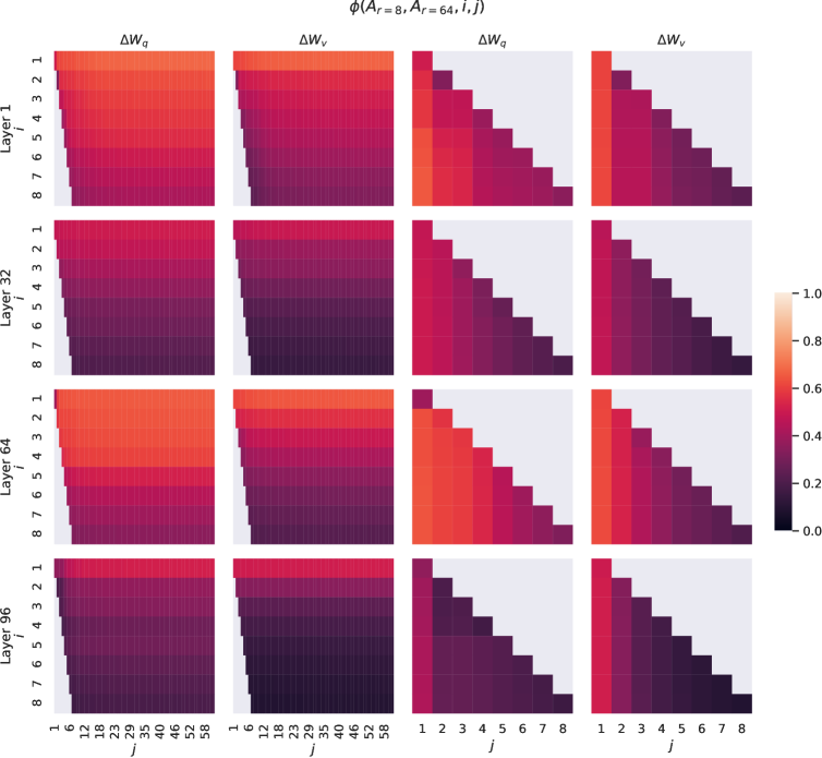
Figure 6: Normalized subspace similarity between the column vectors of Ar=8subscript𝐴𝑟8A_{r=8} and Ar=64subscript𝐴𝑟64A_{r=64} for both Δ​WqΔsubscript𝑊𝑞\Delta W_{q} and Δ​WvΔsubscript𝑊𝑣\Delta W_{v} from the 1st, 32nd, 64th, and 96th layers in a 96-layer Transformer.

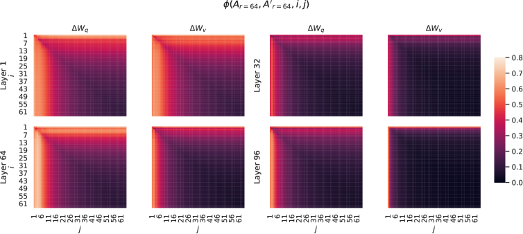
Figure 7: Normalized subspace similarity between the column vectors of Ar=64subscript𝐴𝑟64A_{r=64} from two randomly seeded runs, for both Δ​WqΔsubscript𝑊𝑞\Delta W_{q} and Δ​WvΔsubscript𝑊𝑣\Delta W_{v} from the 1st, 32nd, 64th, and 96th layers in a 96-layer Transformer.

We repeat our experiment on the effect of r𝑟r (Section 7.2) in GPT-2. Using the E2E NLG Challenge dataset as an example, we report the validation loss and test metrics achieved by different choices of r𝑟r after training for 26,000 steps. We present our result in Table 18. The optimal rank for GPT-2 Medium is between 4 and 16 depending on the metric used, which is similar to that for GPT-3 175B. Note that the relationship between model size and the optimal rank for adaptation is still an open question.

Rank r𝑟r

val_loss

BLEU

NIST

METEOR

ROUGE_L

CIDEr

1

1.23

68.72

8.7215

0.4565

0.7052

2.4329

2

1.21

69.17

8.7413

0.4590

0.7052

2.4639

4

1.18

70.38

8.8439

0.4689

0.7186

2.5349

8

1.17

69.57

8.7457

0.4636

0.7196

2.5196

16

1.16

69.61

8.7483

0.4629

0.7177

2.4985

32

1.16

69.33

8.7736

0.4642

0.7105

2.5255

64

1.16

69.24

8.7174

0.4651

0.7180

2.5070

128

1.16

68.73

8.6718

0.4628

0.7127

2.5030

256

1.16

68.92

8.6982

0.4629

0.7128

2.5012

512

1.16

68.78

8.6857

0.4637

0.7128

2.5025

1024

1.17

69.37

8.7495

0.4659

0.7149

2.5090

Table 18: Validation loss and test set metrics on E2E NLG Challenge achieved by LoRA with different rank r𝑟r using GPT-2 Medium. Unlike on GPT-3 where r=1𝑟1r=1 suffices for many tasks, here the performance peaks at r=16𝑟16r=16 for validation loss and r=4𝑟4r=4 for BLEU, suggesting the GPT-2 Medium has a similar intrinsic rank for adaptation compared to GPT-3 175B. Note that some of our hyperparameters are tuned on r=4𝑟4r=4, which matches the parameter count of another baseline, and thus might not be optimal for other choices of r𝑟r.

See Figure 8 for the normalized subspace similarity between W𝑊W and Δ​WΔ𝑊\Delta W with varying r𝑟r.

Note again that Δ​WΔ𝑊\Delta W does not contain the top singular directions of W𝑊W, since the similarity between the top 4 directions in Δ​WΔ𝑊\Delta W and the top-10% of those in W𝑊W barely exceeds 0.2. This gives evidence that Δ​WΔ𝑊\Delta W contains those “task-specific” directions that are otherwise not emphasized in W𝑊W.

An interesting next question to answer, is how “strong” do we need to amplify those task-specific directions, in order for the model adaptation to work well?

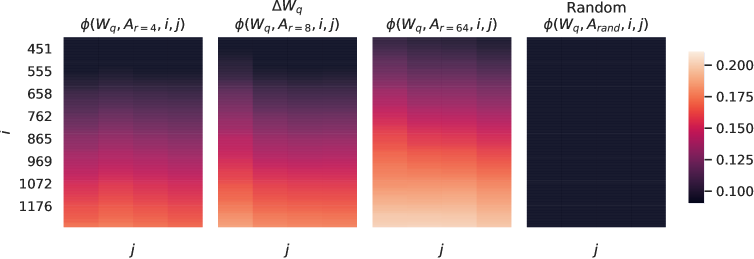
Figure 8: Normalized subspace similarity between the singular directions of Wqsubscript𝑊𝑞W_{q} and those of Δ​WqΔsubscript𝑊𝑞\Delta W_{q} with varying r𝑟r and a random baseline. Δ​WqΔsubscript𝑊𝑞\Delta W_{q} amplifies directions that are important but not emphasized in W𝑊W. Δ​WΔ𝑊\Delta W with a larger r𝑟r tends to pick up more directions that are already emphasized in W𝑊W.

One can naturally consider a feature amplification factor as the ratio ‖Δ​W‖F‖U⊤​W​V⊤‖FsubscriptnormΔ𝑊𝐹subscriptnormsuperscript𝑈top𝑊superscript𝑉top𝐹\frac{\|\Delta W\|_{F}}{\|U^{\top}WV^{\top}\|_{F}}, where U𝑈U and V𝑉V are the left- and right-singular matrices of the SVD decomposition of Δ​WΔ𝑊\Delta W. (Recall U​U⊤​W​V⊤​V𝑈superscript𝑈top𝑊superscript𝑉top𝑉UU^{\top}WV^{\top}V gives the “projection” of W𝑊W onto the subspace spanned by Δ​WΔ𝑊\Delta W.)

Intuitively, when Δ​WΔ𝑊\Delta W mostly contains task-specific directions, this quantity measures how much of them are amplified by Δ​WΔ𝑊\Delta W. As shown in Section 7.3, for r=4𝑟4r=4, this amplification factor is as large as 20. In other words, there are (generally speaking) four feature directions in each layer (out of the entire feature space from the pre-trained model W𝑊W), that need to be amplified by a very large factor 20, in order to achieve our reported accuracy for the downstream specific task. And, one should expect a very different set of feature directions to be amplified for each different downstream task.

One may notice, however, for r=64𝑟64r=64, this amplification factor is only around 2, meaning that most directions learned in Δ​WΔ𝑊\Delta W with r=64𝑟64r=64 are not being amplified by much. This should not be surprising, and in fact gives evidence (once again) that the intrinsic rank needed to represent the “task-specific directions” (thus for model adaptation) is low. In contrast, those directions in the rank-4 version of Δ​WΔ𝑊\Delta W (corresponding to r=4𝑟4r=4) are amplified by a much larger factor 20.

Copyright Privacy Policy

Generated on Thu Mar 7 00:23:07 2024 by LaTeXML